mod_1 = lm(y1 ~ x1, data = anscombe)

plot(anscombe$x1, anscombe$y1); lines(sort(anscombe$x1), predict(mod_1, newdata = list(x1 = sort(anscombe$x1))), col = 'red')
Fitting non-linear regression models
Fitting non-linear regression models can be quite a daunting task from a programming perspective, especially when their complexity increases. Here, we are going to look at four methods of fitting such models.
Fitting linear regression models to data is usually an easy task, since these models have a very simple structure and usually few parameters to optimize. Things get more complicated when one attempts to fit a non-linear model to data, especially when the equation underlying the model has a distinct mechanistic meaning. In such a case, a simple data transformation (e.g. to a logarithmic scale), and fitting a linear model on these transformed data, will not achieve a good model fit or will go against established intellectual consensus. Unfortunately, in practice, non-linear relationships and causalities are more the norm rather than a rarity. Here, we will look a different methods to fit a model on non-linear data, in particular the "x1" and "y1" variables in the anscombe dataset that is included in base R. It is a relatively easy modeling problem, but the methods presented here should be applicable to more complicated problems, as well.
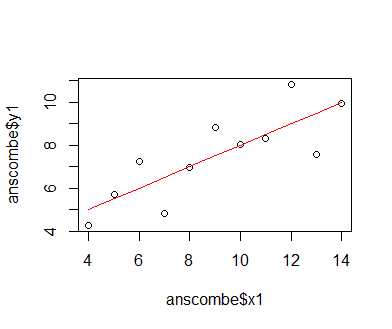
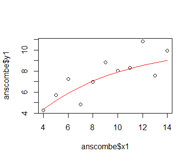
We first fit a classic linear model to the data to demonstrate that this model is not entirely adequate for representing the relationship between x1 and y1. A linear equation describes a simple line within a Cartesian coordinate system, with one parameter, the slope parameter, determining the angle between the abscissa (x axis) of the coordinate system and the line, and the other parameter, the intercept, determining it's offset from the coordinate system's origin. The model is described by the equation f(x) = intercept + slope * x; the variable y1 is thus described as y1 = intercept + slope * x1 + e, where e is the residual error that the model cannot capture. We fit the model using the lm() function in R, which tries to reduce the difference between data and model predictions by iteratively adjusting the slope and intercept using gradient descent. The loss gradient for either parameter is the partial derivative of the loss function (the difference between data and predictions expressed as a function of model-parameter values). The gradient is used to change parameter values in the opposite direction, towards a lower loss. All this happens in background routines of the lm() function. We can see by plotting the model prediction as a line over the actual data points that the model fit is not too well; the data describe a more curved, somewhat asymptotic relationship.
mod_1 = lm(y1 ~ x1, data = anscombe) plot(anscombe$x1, anscombe$y1); lines(sort(anscombe$x1), predict(mod_1, newdata = list(x1 = sort(anscombe$x1))), col = 'red')
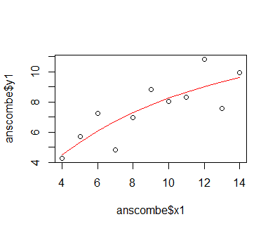
An asymptotic function cannot be defined and fitted using the lm() function, since this is a more complex non-linear function. The function is described by the equation f(x) = maximum * (1 - exp(-slope * x)). Here, "maximum" is actually an asymptotic maximum, a value that the function reaches at an x1 of infinite value, but that is quickly approximated after an initial exponential rise at relatively low values of x1. The exponential-increase par of the function is described by the slope parameter. We fit these parameters to the data using the nls() function, where "nls" stands for non-linear least squares. This means that the loss function is defined by the squared difference between model prediction and observed data, and that partial derivatives of this loss function are used to update maximum and slope to reduce the loss (least squares) via gradient descent. Basically, the fitting procedure is thus equal to that used in lm(). We need to formulate the model equation explicitly this time, though, since nls() can be used for fitting all sorts of non-linear models. In most cases, nls() also requires that the user passes a list of best estimates of intial parameter values that can be guessed from plotting the data. This is because the loss function of such models can be quite complex, and random initial parameter values can lead the gradient-descent algorithm to miss the minimum of the loss function. We can guess the asymptotic maximum to be roughly 10.5, and the slope to be approximately 0.2. The latter is a bit more difficult to guess, since it is part of the exponential part of the model equation. Oftentimes, it is also necessary to standardize the data, so that each variable has a mean of zero and a standard deviation of one. This is especially important in cases where there is more than one predictor variable, and different magnitudes of the value ranges of these data could lead to an unequal weighting of these variables. In the present case, we omit standardizing the data for the moment.
mod_2 = nls(y1 ~ mxm * (1 - exp(-fct * x1)), data = anscombe, start = list(mxm = 10.5, fct = 0.2))
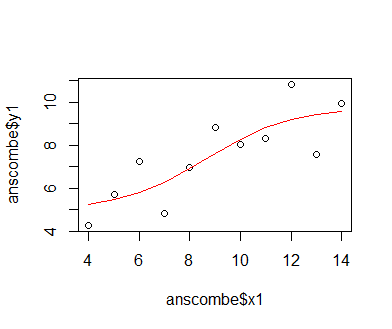
Plotting the predictions of the fitted model as a line together with the actual data shows that the model does represent the relationship between x1 and y1 differently than the simple linear model. Visual inspection indicates that the non-linear model fits the data better, but we should employ the AIC metric to be on the safe side. The AIC metric, called in R via the function AIC(), is, basically speaking, a metric of quality that intgrates the difference of model predictions from the data and the number of model parameters (with fewer parameters being regarded as better, Since less complex models have a lower tendency to over-fit on the data). We find that the AIC value for the non-linear model is lower than that for the linear one, so the asymptotic non-linear model is indeed better suited to describe the data at hand.
plot(anscombe$x1, anscombe$y1); lines(sort(anscombe$x1), predict(mod_2, newdata = list(x1 = sort(anscombe$x1))), col = 'red')

AIC(mod_1)
AIC(mod_2)

In some cases, models can become quite complex; instead of being part of a single equation, parameters may be spread over multiple lines of code that represent a computer simulation of a complex system. Optimization in simulation algorithms can be carried out using the optimr() function in R. Here, we need to go one step further back compared to the nls() function, since we also need to compute the loss ourselves. optimr() requires as inputs a function that returns a scalar loss value, and a list of initial parameter estimates. The function must make require this parameter list as input; accordingly, all parameters used in the function must refer to this input list. The function itself is the algorithm whose parameters we whish to optimize. This function can contain programming language like for-loops or if-else statements, but in the end it is allowed to return only one single value, which is the loss to be minimized. When incorporating, e.g., a model algorithm that loops over discrete time steps, then the function would have to return a loss summed over all time steps. In the present case, we will simply transfer our non-linear model into the optimr synthax for demonstrative purposes. We separate the exponential part of the equation from the rest in order to demonstrate the functions ability to work with multiple lines of code (i.e., an algorithm) instead of a pure equation. We calculate the loss as the squared difference between prediction and original data, summed over all data points.
library('optimr')

opt_func = function(pars){
  outp = exp(-pars[2] * anscombe$x1)
  outp = pars[1] * (1 - outp)

  outp = sum((outp - anscombe$y1)**2)

  return(outp)
}

optimr(c(10.5, 0.2), opt_func)
The output of optimr gives us the optimized parameter estimates, which we will have to insert into the algorithm ourselves; there is no predict() function available for optimr-class objects. Note that optimr() also returns a message about convergence, which indicates whether model optimization was successfull (i.e., the minimum of the loss function was reached) or not. A zero usually indicates successfull convergence. With optimr, you can try several different optimizers for gradient descent. Optimizers are algorithms that try to improve the gradient descent by aggregating information about the result of previous steps of the descent procedure, basically speaking. The optimizer can be specificed via the argument method when calling optimr().
We find that the optimization has converged, so we now insert the optimized parameter values into our original equation to generate predictions. We then plot these along the original data, as before. Unsurprisingly (as our optimization problem is fairly simple), the plot looks exactly like the one generated with the fitted nls-class model. We are unable to compare the fit to the previous model via the AIC function, though, since it does not accept optimr output.
preds = 11.7772005 * (1 - exp(-0.1205108 * sort(anscombe$x1)))

plot(anscombe$x1, anscombe$y1); lines(sort(anscombe$x1), preds, col = 'red')
We can take one step further back and write the optimzation algorithm ourselves using the deriv() function in R. All this function does is calculate the gradients (or first derivatives) of a loss function with respect to parameters involved in the calculation of the loss. This means that parameter updates will have to be performed manually. While in our case this is not a particularly useful tactic, since the nls and optimr functions previously explained work perfectly well, manual gradient calculation can be useful in strongly customized and / or very complex optimization schemes, e.g. optimization in mathematical graphs like neural networks. In these cases, we might prefer to write a custom optimization algorithm, which is not easily supported by the optimr() function. Usage of deriv() requires, however, that we write our code using only very basic mathematical operators and that we omit any programming operators like sum() or mean().
This means that we need to calculate the squared difference between observation and prediction for every single data point, and then add up all single squared errors. In the following lines of code, a prediction and its squared difference from the observation (y_1 to y_11; anscombe consists of eleven observations) is calculated for every data point using the asymptotic function f(x) = maximum * (1 - exp(-slope * x)) described above. As in the nls example, the aymptotic maximum is referred to as mxm, and the slope of the exponential part of the function is named fct. The eleven losses are summed using simple addition operations, omitting any programming "parlance". This formulation is embedded as the first argument in the deriv() function. The second argument is a list of the names of those parameters for which we want to calculate partial derivatives (i.e. loss gradients). deriv now takes the provided input to generate unevaluated R expressions (i.e. inert lines of R code) that will return the partial derivatives once they are evaluated by a specific function call.
dv = deriv( ~
               (y_1 - mxm * (1 - exp(-fct * inp_1)))**2 +
               (y_2 - mxm * (1 - exp(-fct * inp_2)))**2 +
               (y_3 - mxm * (1 - exp(-fct * inp_3)))**2 +
               (y_4 - mxm * (1 - exp(-fct * inp_4)))**2 +
               (y_5 - mxm * (1 - exp(-fct * inp_5)))**2 +
               (y_6 - mxm * (1 - exp(-fct * inp_6)))**2 +
               (y_7 - mxm * (1 - exp(-fct * inp_7)))**2 +
               (y_8 - mxm * (1 - exp(-fct * inp_8)))**2 +
               (y_9 - mxm * (1 - exp(-fct * inp_9)))**2 +
               (y_10 - mxm * (1 - exp(-fct * inp_10)))**2 +
               (y_11 - mxm * (1 - exp(-fct * inp_11)))**2,

             c('mxm', 'fct')
)
Before we can evaluate the expression, we need to assign values to the data and parameters that appear in the expression. These are the parameters mxm and fct and the x-values inp_1 to inp_11 and corresponding y-values y_1 to y_11. These must, of course, be drawn from the anscombe dataset. To speed up coding, this is done here using the lapply() function as shown below. To the unexperienced R programmer, this may come off as somewhat cryptic, but bascially, all it does are the operations
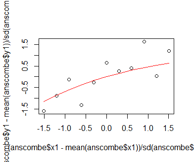
y_i = (anscombe$y1[i] - mean(anscombe$y1)) / sd(anscombe$y1), for every i in one to eleven; the same operation is performed for the x1 variable in anscombe. The subtraction of the mean and division by the standard deviation are the typical standardization procedure that scale the variables x1 and y1 to similar magnitudes, which often helps in the optimzation process. The parameters are intialized with the values 1.4 (mxm) and 0.4 (fct), which are different from the intial values used in the previous optimizer functions, since we arenow working with the standardized data. Plotting the standardized data reveals that the asymptotic maximum is approximately 1.4; the value 0.4 for the slope of the exponential component of the model function is derived from manual experimentation on model fit.
lapply(seq(1,11,1), function(i){eval(parse(text = paste0('assign("y_', i, '", (anscombe$y1[',i,'] - mean(anscombe$y1)) / sd(anscombe$y1), .GlobalEnv)')))})
lapply(seq(1,11,1), function(i){eval(parse(text = paste0('assign("inp_', i, '", (anscombe$x1[',i,'] - mean(anscombe$x1)) / sd(anscombe$x1), .GlobalEnv)')))})

plot((anscombe$x1 - mean(anscombe$x1)) / sd(anscombe$x1), (anscombe$y1 - mean(anscombe$y1)) / sd(anscombe$y1))

mxm = 1.4
fct = 0.4

lines(sort((anscombe$x1 - mean(anscombe$x1)) / sd(anscombe$x1)),
      mxm * (1 - exp(-fct * sort((anscombe$x1 - mean(anscombe$x1)) / sd(anscombe$x1)))), col = 'red')
Having defined the input data, observations against which predictions are to be compared, and initial parameter values, we can now evaluate the deriv expression to obtain our first set of derivatives of the loss function with respect to parameters mxm and fct. We evaluate the expression using the common eval() function, which can be used to evaluate (think "activate") any inert expression in R. We obtain a list of values containing the loss itself and the derivatives, or loss-function gradients. Now, we use these to update our initial parameter guess values. Essentially, we move the parameter values in the opposite direction of the gradients by a step of a certain size. This step size is called the learning rate, which we must fix to a value we assume suitable for effective optimization. In the current example, we set it to 0.001. The gradients are then updated according to the equation parameter_new = parameter - learning_rate * gradient.
grds = eval(dv)
loss = grds[1]
grds
grds = attributes(grds)
grds = unlist(grds)

lr = 1e-3

mxm = mxm - lr * grds[1]
fct = fct - lr * grds[2]

loss_list = loss
We now iterate this set of procedures - calculating loss and gradients, and updating the parameters using the gradients - for several times in order to approach the global minimum of the loss function. Close to that minimum, gradients will become shallow, and parameter updates will become marginal. We also record the loss at each step to later visualize the optimization procedure. Using the deriv function, we can only make a good guess as to whether we have truly arrived at a minimum of the loss function, and not some undesirable property like a saddle point, an area also characterized by shallow loss gradients. This is normally assessed using the properties of the Hessian matrix, though the calculation of that matrix is beyond the content of this tutorial. An unsuitable state of the Hessian matrix, i.e. a failure of optimization convergence, happens mostly in very complex or miss-specified models. Neither of these are attributes of our optimization problem, so we can be fairly confident that we will have little trouble using deriv for optimization here.
for(i in 1:60){
  grds = eval(dv)
  loss = grds[1]
  grds = attributes(grds)[2]
  grds = unlist(grds)

  loss_list = c(loss_list, loss)

  mxm = mxm - lr * grds[1]
  fct = fct - lr * grds[2]
}
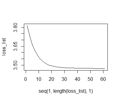
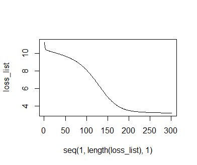
After the iterations have been completed, we plot the recorded losses against the iteration index. We find that the loss decreases and nears an asymptote. This indicates that the optimization has worked out well, and that further iterations will yield only very marginal improvements. Thus, there is not really any point to continuing the optimization. Like before, we also plot the data and the model predictions. We need to backtransform the model predictions from the standardized scale to the original scale of the y1-data, so we need to multiply them with the standard deviation of y1 and then add the mean of y1. We find that the curve of model predictions is similar, but not identical to the one obtained from the optimr-based optimization. This is likely due to the fact that we did not use a specific optimizer algorithm, and that we did not use a formal criterion for stopping the optimization. Though not shown here, the final loss of the deriv-based optimization is a little lower than that returned by the optimr-based optimization.
plot(seq(1,length(loss_list),1), loss_list, type = 'l')

preds = mxm * (1 - exp(-fct * (sort(anscombe$x1) - mean(anscombe$x1)) / sd(anscombe$x1)))
preds = mean(anscombe$y1) + (sd(anscombe$y1) * preds)

plot(anscombe$x1, anscombe$y1); lines(sort(anscombe$x1), preds, col = 'red')
As a final method,we can invoke the power of deep neural networks (DNNs) as function approximators for our optimization problem. DNNs are highly-parameterized directed mathematical graphs. Though there is no mechanistic reasoning to the architecture of the DNN (other than the coincidental similarity to the arrangement of neurons in the animal brain), the output of a DNN can theoretically approximate the output of any simpler function. One constraint is that the architecture of the DNN must be specified without really knowing how much complexity is required. Designing DNNs is rather a matter of experience than of adherence to rules. In our case, the method can help us find out whether the asymptotic function is really the best mechanistic description of our data. We will utilize a realtively simple design given the simplicity of our optimization problem (still, the DNN will contain 22 parameters (see below)).

The construction and training of DNNs via the deriv() function in R has been discussed in depth in a previous article. We do make two notable differences to the approach described there: first, we optimize by calculating the loss over all data points at once in each iteration, unlike using only one data point per parameter-update. This, of course, means that our code becomes quite long. Second, we have a regression, not a classification problem at hand. Therefore, i) our DNN has only one output node, ii) we do not apply a softmax activation function on the output of that node, and iii) our loss is the squared difference between observation and prediction, summed over all data points, instead of categorical cross-entropy. The DNN itself consists of a one-dimensional input layer, two consecutive hidden layers with three nodes and sigmoid activation each, and a one-dimensional output layer. Bearing these changes in mind, the rest of the procedures is pretty much identical to those described in the earlier article, and will not be described again here.
dv = deriv( ~
(y_1 - (
sl_3_n1_a * (1 / (1 + exp(-
sl_2_n1_a * (1 / (1 + exp(-(sl_1_n1 * inp_1 + int_1_n1)))) +
sl_2_n1_b * (1 / (1 + exp(-(sl_1_n2 * inp_1 + int_1_n2)))) +
sl_2_n1_c * (1 / (1 + exp(-(sl_1_n3 * inp_1 + int_1_n3)))) +
int_2_n1))) +
sl_3_n1_b * (1 / (1 + exp(-
sl_2_n2_a * (1 / (1 + exp(-(sl_1_n1 * inp_1 + int_1_n1)))) +
sl_2_n2_b * (1 / (1 + exp(-(sl_1_n2 * inp_1 + int_1_n2)))) +
sl_2_n2_c * (1 / (1 + exp(-(sl_1_n3 * inp_1 + int_1_n3)))) +
int_2_n2))) +
sl_3_n1_c * (1 / (1 + exp(-
sl_2_n3_a * (1 / (1 + exp(-(sl_1_n1 * inp_1 + int_1_n1)))) +
sl_2_n3_b * (1 / (1 + exp(-(sl_1_n2 * inp_1 + int_1_n2)))) +
sl_2_n3_c * (1 / (1 + exp(-(sl_1_n3 * inp_1 + int_1_n3)))) +
int_2_n3))) +
int_3_n1
))**2 +
(y_2 - (
sl_3_n1_a * (1 / (1 + exp(-
sl_2_n1_a * (1 / (1 + exp(-(sl_1_n1 * inp_2 + int_1_n1)))) +
sl_2_n1_b * (1 / (1 + exp(-(sl_1_n2 * inp_2 + int_1_n2)))) +
sl_2_n1_c * (1 / (1 + exp(-(sl_1_n3 * inp_2 + int_1_n3)))) +
int_2_n1))) +
sl_3_n1_b * (1 / (1 + exp(-
sl_2_n2_a * (1 / (1 + exp(-(sl_1_n1 * inp_2 + int_1_n1)))) +
sl_2_n2_b * (1 / (1 + exp(-(sl_1_n2 * inp_2 + int_1_n2)))) +
sl_2_n2_c * (1 / (1 + exp(-(sl_1_n3 * inp_2 + int_1_n3)))) +
int_2_n2))) +
sl_3_n1_c * (1 / (1 + exp(-
sl_2_n3_a * (1 / (1 + exp(-(sl_1_n1 * inp_2 + int_1_n1)))) +
sl_2_n3_b * (1 / (1 + exp(-(sl_1_n2 * inp_2 + int_1_n2)))) +
sl_2_n3_c * (1 / (1 + exp(-(sl_1_n3 * inp_2 + int_1_n3)))) +
int_2_n3))) +
int_3_n1
))**2 +
(y_3 - (
sl_3_n1_a * (1 / (1 + exp(-
sl_2_n1_a * (1 / (1 + exp(-(sl_1_n1 * inp_3 + int_1_n1)))) +
sl_2_n1_b * (1 / (1 + exp(-(sl_1_n2 * inp_3 + int_1_n2)))) +
sl_2_n1_c * (1 / (1 + exp(-(sl_1_n3 * inp_3 + int_1_n3)))) +
int_2_n1))) +
sl_3_n1_b * (1 / (1 + exp(-
sl_2_n2_a * (1 / (1 + exp(-(sl_1_n1 * inp_3 + int_1_n1)))) +
sl_2_n2_b * (1 / (1 + exp(-(sl_1_n2 * inp_3 + int_1_n2)))) +
sl_2_n2_c * (1 / (1 + exp(-(sl_1_n3 * inp_3 + int_1_n3)))) +
int_2_n2))) +
sl_3_n1_c * (1 / (1 + exp(-
sl_2_n3_a * (1 / (1 + exp(-(sl_1_n1 * inp_3 + int_1_n1)))) +
sl_2_n3_b * (1 / (1 + exp(-(sl_1_n2 * inp_3 + int_1_n2)))) +
sl_2_n3_c * (1 / (1 + exp(-(sl_1_n3 * inp_3 + int_1_n3)))) +
int_2_n3))) +
int_3_n1
))**2 +
(y_4 - (
sl_3_n1_a * (1 / (1 + exp(-
sl_2_n1_a * (1 / (1 + exp(-(sl_1_n1 * inp_4 + int_1_n1)))) +
sl_2_n1_b * (1 / (1 + exp(-(sl_1_n2 * inp_4 + int_1_n2)))) +
sl_2_n1_c * (1 / (1 + exp(-(sl_1_n3 * inp_4 + int_1_n3)))) +
int_2_n1))) +
sl_3_n1_b * (1 / (1 + exp(-
sl_2_n2_a * (1 / (1 + exp(-(sl_1_n1 * inp_4 + int_1_n1)))) +
sl_2_n2_b * (1 / (1 + exp(-(sl_1_n2 * inp_4 + int_1_n2)))) +
sl_2_n2_c * (1 / (1 + exp(-(sl_1_n3 * inp_4 + int_1_n3)))) +
int_2_n2))) +
sl_3_n1_c * (1 / (1 + exp(-
sl_2_n3_a * (1 / (1 + exp(-(sl_1_n1 * inp_4 + int_1_n1)))) +
sl_2_n3_b * (1 / (1 + exp(-(sl_1_n2 * inp_4 + int_1_n2)))) +
sl_2_n3_c * (1 / (1 + exp(-(sl_1_n3 * inp_4 + int_1_n3)))) +
int_2_n3))) +
int_3_n1
))**2 +
(y_5 - (
sl_3_n1_a * (1 / (1 + exp(-
sl_2_n1_a * (1 / (1 + exp(-(sl_1_n1 * inp_5 + int_1_n1)))) +
sl_2_n1_b * (1 / (1 + exp(-(sl_1_n2 * inp_5 + int_1_n2)))) +
sl_2_n1_c * (1 / (1 + exp(-(sl_1_n3 * inp_5 + int_1_n3)))) +
int_2_n1))) +
sl_3_n1_b * (1 / (1 + exp(-
sl_2_n2_a * (1 / (1 + exp(-(sl_1_n1 * inp_5 + int_1_n1)))) +
sl_2_n2_b * (1 / (1 + exp(-(sl_1_n2 * inp_5 + int_1_n2)))) +
sl_2_n2_c * (1 / (1 + exp(-(sl_1_n3 * inp_5 + int_1_n3)))) +
int_2_n2))) +
sl_3_n1_c * (1 / (1 + exp(-
sl_2_n3_a * (1 / (1 + exp(-(sl_1_n1 * inp_5 + int_1_n1)))) +
sl_2_n3_b * (1 / (1 + exp(-(sl_1_n2 * inp_5 + int_1_n2)))) +
sl_2_n3_c * (1 / (1 + exp(-(sl_1_n3 * inp_5 + int_1_n3)))) +
int_2_n3))) +
int_3_n1
))**2 +
(y_6 - (
sl_3_n1_a * (1 / (1 + exp(-
sl_2_n1_a * (1 / (1 + exp(-(sl_1_n1 * inp_6 + int_1_n1)))) +
sl_2_n1_b * (1 / (1 + exp(-(sl_1_n2 * inp_6 + int_1_n2)))) +
sl_2_n1_c * (1 / (1 + exp(-(sl_1_n3 * inp_6 + int_1_n3)))) +
int_2_n1))) +
sl_3_n1_b * (1 / (1 + exp(-
sl_2_n2_a * (1 / (1 + exp(-(sl_1_n1 * inp_6 + int_1_n1)))) +
sl_2_n2_b * (1 / (1 + exp(-(sl_1_n2 * inp_6 + int_1_n2)))) +
sl_2_n2_c * (1 / (1 + exp(-(sl_1_n3 * inp_6 + int_1_n3)))) +
int_2_n2))) +
sl_3_n1_c * (1 / (1 + exp(-
sl_2_n3_a * (1 / (1 + exp(-(sl_1_n1 * inp_6 + int_1_n1)))) +
sl_2_n3_b * (1 / (1 + exp(-(sl_1_n2 * inp_6 + int_1_n2)))) +
sl_2_n3_c * (1 / (1 + exp(-(sl_1_n3 * inp_6 + int_1_n3)))) +
int_2_n3))) +
int_3_n1
))**2 +
(y_7 - (
sl_3_n1_a * (1 / (1 + exp(-
sl_2_n1_a * (1 / (1 + exp(-(sl_1_n1 * inp_7 + int_1_n1)))) +
sl_2_n1_b * (1 / (1 + exp(-(sl_1_n2 * inp_7 + int_1_n2)))) +
sl_2_n1_c * (1 / (1 + exp(-(sl_1_n3 * inp_7 + int_1_n3)))) +
int_2_n1))) +
sl_3_n1_b * (1 / (1 + exp(-
sl_2_n2_a * (1 / (1 + exp(-(sl_1_n1 * inp_7 + int_1_n1)))) +
sl_2_n2_b * (1 / (1 + exp(-(sl_1_n2 * inp_7 + int_1_n2)))) +
sl_2_n2_c * (1 / (1 + exp(-(sl_1_n3 * inp_7 + int_1_n3)))) +
int_2_n2))) +
sl_3_n1_c * (1 / (1 + exp(-
sl_2_n3_a * (1 / (1 + exp(-(sl_1_n1 * inp_7 + int_1_n1)))) +
sl_2_n3_b * (1 / (1 + exp(-(sl_1_n2 * inp_7 + int_1_n2)))) +
sl_2_n3_c * (1 / (1 + exp(-(sl_1_n3 * inp_7 + int_1_n3)))) +
int_2_n3))) +
int_3_n1
))**2 +
(y_8 - (
sl_3_n1_a * (1 / (1 + exp(-
sl_2_n1_a * (1 / (1 + exp(-(sl_1_n1 * inp_8 + int_1_n1)))) +
sl_2_n1_b * (1 / (1 + exp(-(sl_1_n2 * inp_8 + int_1_n2)))) +
sl_2_n1_c * (1 / (1 + exp(-(sl_1_n3 * inp_8 + int_1_n3)))) +
int_2_n1))) +
sl_3_n1_b * (1 / (1 + exp(-
sl_2_n2_a * (1 / (1 + exp(-(sl_1_n1 * inp_8 + int_1_n1)))) +
sl_2_n2_b * (1 / (1 + exp(-(sl_1_n2 * inp_8 + int_1_n2)))) +
sl_2_n2_c * (1 / (1 + exp(-(sl_1_n3 * inp_8 + int_1_n3)))) +
int_2_n2))) +
sl_3_n1_c * (1 / (1 + exp(-
sl_2_n3_a * (1 / (1 + exp(-(sl_1_n1 * inp_8 + int_1_n1)))) +
sl_2_n3_b * (1 / (1 + exp(-(sl_1_n2 * inp_8 + int_1_n2)))) +
sl_2_n3_c * (1 / (1 + exp(-(sl_1_n3 * inp_8 + int_1_n3)))) +
int_2_n3))) +
int_3_n1
))**2 +
(y_9 - (
sl_3_n1_a * (1 / (1 + exp(-
sl_2_n1_a * (1 / (1 + exp(-(sl_1_n1 * inp_9 + int_1_n1)))) +
sl_2_n1_b * (1 / (1 + exp(-(sl_1_n2 * inp_9 + int_1_n2)))) +
sl_2_n1_c * (1 / (1 + exp(-(sl_1_n3 * inp_9 + int_1_n3)))) +
int_2_n1))) +
sl_3_n1_b * (1 / (1 + exp(-
sl_2_n2_a * (1 / (1 + exp(-(sl_1_n1 * inp_9 + int_1_n1)))) +
sl_2_n2_b * (1 / (1 + exp(-(sl_1_n2 * inp_9 + int_1_n2)))) +
sl_2_n2_c * (1 / (1 + exp(-(sl_1_n3 * inp_9 + int_1_n3)))) +
int_2_n2))) +
sl_3_n1_c * (1 / (1 + exp(-
sl_2_n3_a * (1 / (1 + exp(-(sl_1_n1 * inp_9 + int_1_n1)))) +
sl_2_n3_b * (1 / (1 + exp(-(sl_1_n2 * inp_9 + int_1_n2)))) +
sl_2_n3_c * (1 / (1 + exp(-(sl_1_n3 * inp_9 + int_1_n3)))) +
int_2_n3))) +
int_3_n1
))**2 +
(y_10 - (
sl_3_n1_a * (1 / (1 + exp(-
sl_2_n1_a * (1 / (1 + exp(-(sl_1_n1 * inp_10 + int_1_n1)))) +
sl_2_n1_b * (1 / (1 + exp(-(sl_1_n2 * inp_10 + int_1_n2)))) +
sl_2_n1_c * (1 / (1 + exp(-(sl_1_n3 * inp_10 + int_1_n3)))) +
int_2_n1))) +
sl_3_n1_b * (1 / (1 + exp(-
sl_2_n2_a * (1 / (1 + exp(-(sl_1_n1 * inp_10 + int_1_n1)))) +
sl_2_n2_b * (1 / (1 + exp(-(sl_1_n2 * inp_10 + int_1_n2)))) +
sl_2_n2_c * (1 / (1 + exp(-(sl_1_n3 * inp_10 + int_1_n3)))) +
int_2_n2))) +
sl_3_n1_c * (1 / (1 + exp(-
sl_2_n3_a * (1 / (1 + exp(-(sl_1_n1 * inp_10 + int_1_n1)))) +
sl_2_n3_b * (1 / (1 + exp(-(sl_1_n2 * inp_10 + int_1_n2)))) +
sl_2_n3_c * (1 / (1 + exp(-(sl_1_n3 * inp_10 + int_1_n3)))) +
int_2_n3))) +
int_3_n1
))**2 +
(y_11 - (
sl_3_n1_a * (1 / (1 + exp(-
sl_2_n1_a * (1 / (1 + exp(-(sl_1_n1 * inp_11 + int_1_n1)))) +
sl_2_n1_b * (1 / (1 + exp(-(sl_1_n2 * inp_11 + int_1_n2)))) +
sl_2_n1_c * (1 / (1 + exp(-(sl_1_n3 * inp_11 + int_1_n3)))) +
int_2_n1))) +
sl_3_n1_b * (1 / (1 + exp(-
sl_2_n2_a * (1 / (1 + exp(-(sl_1_n1 * inp_11 + int_1_n1)))) +
sl_2_n2_b * (1 / (1 + exp(-(sl_1_n2 * inp_11 + int_1_n2)))) +
sl_2_n2_c * (1 / (1 + exp(-(sl_1_n3 * inp_11 + int_1_n3)))) +
int_2_n2))) +
sl_3_n1_c * (1 / (1 + exp(-
sl_2_n3_a * (1 / (1 + exp(-(sl_1_n1 * inp_11 + int_1_n1)))) +
sl_2_n3_b * (1 / (1 + exp(-(sl_1_n2 * inp_11 + int_1_n2)))) +
sl_2_n3_c * (1 / (1 + exp(-(sl_1_n3 * inp_11 + int_1_n3)))) +
int_2_n3))) +
int_3_n1
))**2
,
c('sl_1_n1', 'sl_1_n2', 'sl_1_n3',
'sl_2_n1_a', 'sl_2_n1_b', 'sl_2_n1_c',
'sl_2_n2_a', 'sl_2_n2_b', 'sl_2_n2_c',
'sl_2_n3_a', 'sl_2_n3_b', 'sl_2_n3_c',
'sl_3_n1_a', 'sl_3_n1_b', 'sl_3_n1_c',
'int_1_n1', 'int_1_n2', 'int_1_n3',
'int_2_n1', 'int_2_n2', 'int_3_n3',
'int_3_n1')
)
set.seed(123)
rands = rnorm(22)
sl_1_n1 = rands[1]
sl_1_n2 = rands[2]
sl_1_n3 = rands[3]
sl_2_n1_a = rands[4]
sl_2_n1_b = rands[5]
sl_2_n1_c = rands[6]
sl_2_n2_a = rands[7]
sl_2_n2_b = rands[8]
sl_2_n2_c = rands[9]
sl_2_n3_a = rands[10]
sl_2_n3_b = rands[11]
sl_2_n3_c = rands[12]
sl_3_n1_a = rands[13]
sl_3_n1_b = rands[14]
sl_3_n1_c = rands[15]
int_1_n1 = rands[16]
int_1_n2 = rands[17]
int_1_n3 = rands[18]
int_2_n1 = rands[19]
int_2_n2 = rands[20]
int_2_n3 = rands[21]
int_3_n1 = rands[22]
grds = eval(dv)
loss = grds[1]
grds
grds = attributes(grds)
grds = unlist(grds)
lr = 1e-2
sl_1_n1 = sl_1_n1 - lr * grds[1]
sl_1_n2 = sl_1_n2 - lr * grds[2]
sl_1_n3 = sl_1_n3 - lr * grds[3]
sl_2_n1_a = sl_2_n1_a - lr * grds[4]
sl_2_n1_b = sl_2_n1_b - lr * grds[5]
sl_2_n1_c = sl_2_n1_c - lr * grds[6]
sl_2_n2_a = sl_2_n2_a - lr * grds[7]
sl_2_n2_b = sl_2_n2_b - lr * grds[8]
sl_2_n2_c = sl_2_n2_c - lr * grds[9]
sl_2_n3_a = sl_2_n3_a - lr * grds[10]
sl_2_n3_b = sl_2_n3_b - lr * grds[11]
sl_2_n3_c = sl_2_n3_c - lr * grds[12]
sl_3_n1_a = sl_3_n1_a - lr * grds[13]
sl_3_n1_b = sl_3_n1_b - lr * grds[14]
sl_3_n1_c = sl_3_n1_c - lr * grds[15]
int_1_n1 = int_1_n1 - lr * grds[16]
int_1_n2 = int_1_n2 - lr * grds[17]
int_1_n3 = int_1_n3 - lr * grds[18]
int_2_n1 = int_2_n1 - lr * grds[19]
int_2_n2 = int_2_n2 - lr * grds[20]
int_2_n3 = int_2_n3 - lr * grds[21]
int_3_n1 = int_3_n1 - lr * grds[22]
loss_list = loss
for(i in 1:300){
grds = eval(dv)
loss = grds[1]
grds = attributes(grds)[2]
grds = unlist(grds)
loss_list = c(loss_list, loss)
sl_1_n1 = sl_1_n1 - lr * grds[1]
sl_1_n2 = sl_1_n2 - lr * grds[2]
sl_1_n3 = sl_1_n3 - lr * grds[3]
sl_2_n1_a = sl_2_n1_a - lr * grds[4]
sl_2_n1_b = sl_2_n1_b - lr * grds[5]
sl_2_n1_c = sl_2_n1_c - lr * grds[6]
sl_2_n2_a = sl_2_n2_a - lr * grds[7]
sl_2_n2_b = sl_2_n2_b - lr * grds[8]
sl_2_n2_c = sl_2_n2_c - lr * grds[9]
sl_2_n3_a = sl_2_n3_a - lr * grds[10]
sl_2_n3_b = sl_2_n3_b - lr * grds[11]
sl_2_n3_c = sl_2_n3_c - lr * grds[12]
sl_3_n1_a = sl_3_n1_a - lr * grds[13]
sl_3_n1_b = sl_3_n1_b - lr * grds[14]
sl_3_n1_c = sl_3_n1_c - lr * grds[15]
int_1_n1 = int_1_n1 - lr * grds[16]
int_1_n2 = int_1_n2 - lr * grds[17]
int_1_n3 = int_1_n3 - lr * grds[18]
int_2_n1 = int_2_n1 - lr * grds[19]
int_2_n2 = int_2_n2 - lr * grds[20]
int_2_n3 = int_2_n3 - lr * grds[21]
int_3_n1 = int_3_n1 - lr * grds[22]
}
Plotting the loss trajectory, we find that loss does decrease and reaches an asymptote, though curiously, the decrease is intitially more sigmoidal in shape than the exponential patterns observed earlier. Plotting of the predictions reveals not the asymptotic function assumed in our earlier optimization attempts, but a slightly sigmoidal shape. According to loss summed over all data points, this function is a markedly better fit to the data than the original asymptotic function. We could now use this information to construct and fit a "true" sigmoidal function using the nls or optimr functions. This will in many cases be preferrable over using the DNN directly for making predictions on new data, since a mechanistic understanding of processes is often as much desired as the ability to make accurate predictions.
plot(seq(1,length(loss_list),1), loss_list, type = 'l')

prds_list = NULL

for(i in 1:11){
  eval(parse(text = paste0("
               prds_list[length(prds_list)+1] =
                  sl_3_n1_a * (1 / (1 + exp(-
                                           sl_2_n1_a * (1 / (1 + exp(-(sl_1_n1 * inp_",i," + int_1_n1)))) +
                                           sl_2_n1_b * (1 / (1 + exp(-(sl_1_n2 * inp_",i," + int_1_n2)))) +
                                           sl_2_n1_c * (1 / (1 + exp(-(sl_1_n3 * inp_",i," + int_1_n3)))) +
                                           int_2_n1))) +
                 sl_3_n1_b * (1 / (1 + exp(-
                                           sl_2_n2_a * (1 / (1 + exp(-(sl_1_n1 * inp_",i," + int_1_n1)))) +
                                           sl_2_n2_b * (1 / (1 + exp(-(sl_1_n2 * inp_",i," + int_1_n2)))) +
                                           sl_2_n2_c * (1 / (1 + exp(-(sl_1_n3 * inp_",i," + int_1_n3)))) +
                                           int_2_n2))) +
                 sl_3_n1_c * (1 / (1 + exp(-
                                           sl_2_n3_a * (1 / (1 + exp(-(sl_1_n1 * inp_",i," + int_1_n1)))) +
                                           sl_2_n3_b * (1 / (1 + exp(-(sl_1_n2 * inp_",i," + int_1_n2)))) +
                                           sl_2_n3_c * (1 / (1 + exp(-(sl_1_n3 * inp_",i," + int_1_n3)))) +
                                           int_2_n3))) +
                 int_3_n1
               ")))
}

preds = mean(anscombe$y1) + (sd(anscombe$y1) * prds_list)

sorted_inds = sort(anscombe$x1, index.return=T)$ix

plot(anscombe$x1, anscombe$y1)
lines(sort(anscombe$x1), preds[sorted_inds], col = 'red')
We have thus discussed several methods for fitting non-linear models. The best choice will depend on the complexity of the optimization problem, with the deriv function offering maximum flexibility in the design and training of the model. We have also found that using deep neural networks in an exploratory manner can help decide on the nature of the non-linear function to be fitted.