Building a deep neural network from scratch
Deep neural networks for classification or regression are typically constructed via the Keras API in Python, which is so user-friendly that it is essentially a blackbox. Here we will look at a much less opaque approach using the deriv() function in R.
Deep neural networks (DNNs) are at the core of modern classifier systems colloquially referred to as devices using "Artificial Intelligence". Yet the inner mechanisms of the models behind these device are shrouded in mystery to many. This may be also founded in the fact that with the availability of modern application-programming interfaces (APIs) like Keras, one does not need to have intricate knowledge about the optimization of such models. Here, we are going to build a simple DNN on our own using only the deriv() function in R. This allows us to construct all steps in the assembly and training of DNNs on our own, rather than relying on the "black-box" API. Please be aware that this article is not intended to teach the inner mechanisms of DNNs and of their training; we will only look at the implementation of model construction and training here.
Deriv() is a basic function in R that calculates the derivative of any function with respect to parameters contained within this function. Calculating derivatives is of importance in training a DNN, as in most Machine-Learning models. What is calculated are actually the gradients of the loss function of the DNN model with respect to its parameters, and the gradient of any function is given by its first derivative. Functions passed to deriv() can be of arbitrary complexity, but can only contain relatively basic mathematical operations; more specific functions like sum() or mean() cannot be used.
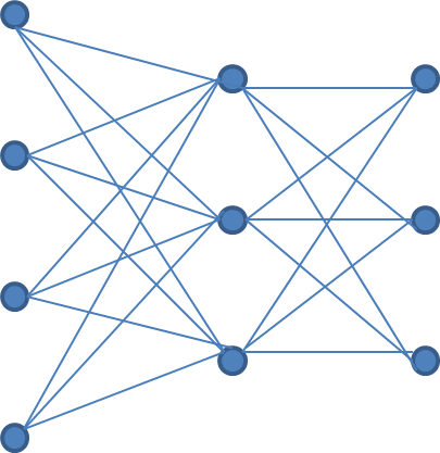
Let us now build our DNN within the context of the deriv() function. In particular, what we actually construct is the loss function that takes an observation and the DNN itself, which calculates the prediction, and yields a scalar value. This scalar loss is the key to calculating the partial derivatives with respect to the parameters in the DNN. Our DNN will have three layers: One input layer that receives a four-dimensional input, one hidden layer with three nodes, and one output layer with three nodes. The input and first hidden layers will be connected with 4 * 3 = 12 weights, plus three biases, one for each node in the first hidden layer. The first hidden layer and the output layer (i.e. the second hidden layer) will be connected with 3 * 3 = 9 weights plus three biases, one for each node in the output layer. Formally, we will treat each bias as an additional weight that is applied to a pseudo-input-dimension or to a pseudo-node of value 1. The summed products of input data and weights, plus the bias, will be activated with a sigmoid function in the first hidden layer, and with a softmax function in the output layer. The softmax function simply ensures that the outputs of all nodes in the final layer sum to 1. The final output of the DNN, that is, a vector of three values that sum to one, will be compared to the ground truth, a one-hot-encoded vector of three values, i.e. a vector with two zeros and one one.
Since deriv() allows no usage of aggregative operators, like sum(), and since we do not wanter to enter the subject of matrix calculations at this point, we will have to write a lot of replications in our code in order to calculate the final scalar loss, from the multivariate DNN output and ground truth. We will look at single expressions first, and then gradually piece everything together. We begin with the calculations for one single node of the first hidden layer: Since we have four-dimensional input data, we have four input values, termed in1a to in1d. Each of these is multiplied with one parameter, or weight, as in x1a1 * in1a. x1a1 to x1d1 are the names of the weights. The products are added. Finally, we add the bias, which is, in this example, formally treated like a weight, hence it is multiplied with a scalar 1 instead of an input value. The bias is called x1e1. The product of bias and scalar 1 is added to the previous addition operations. Finally, The entire sum is activated with a sigmoid function of the form 1 / (1 + exp(-x)), where x is the sum of input-weight multiplications and the bias.
1/(1+exp(-(x1a1 * in1a + x1b1 * in1b + x1c1 * in1c + x1d1 * in1d + x1e1 * 1)))
Since we have three nodes, this procedure must be repeated for each node. Note that the weights for each node are unique, as is the bias. So, for the second node, we have weights x1a2 to x1d2, and for the final node we have weights x1a3 to x1d3. The inputs are the same for every node, however, since every input value is connected to every node in the first hidden layer. So we still have in1a to in1d for the second and third nodes.
1/(1+exp(-(x1a1 * in1a + x1b1 * in1b + x1c1 * in1c + x1d1 * in1d + x1e1 * 1)))
1/(1+exp(-(x1a2 * in1a + x1b2 * in1b + x1c2 * in1c + x1d2 * in1d + x1e2 * 1)))
1/(1+exp(-(x1a3 * in1a + x1b3 * in1b + x1c3 * in1c + x1d3 * in1d + x1e3 * 1)))
Now, we come to the second hidden layer, or output layer. This layer, like the first hidden layer, has three nodes. In each node, the output of each of the nodes of the previous layer, i.e. the result of the sigmoid activation, is multiplied with one weight. For the first node in the output layer, these are the weights x2a1 to x2c1. Again, the products are added. A bias, x2d1, which is again treated as a weight and thus multiplied with a scalar 1, is added, as well.
x2a1 * 1/(1+exp(-(x1a1 * in1a + x1b1 * in1b + x1c1 * in1c + x1d1 * in1d + x1e1 * 1))) +
x2b1 * 1/(1+exp(-(x1a2 * in1a + x1b2 * in1b + x1c2 * in1c + x1d2 * in1d + x1e2 * 1))) +
x2c1 * 1/(1+exp(-(x1a3 * in1a + x1b3 * in1b + x1c3 * in1c + x1d3 * in1d + x1e3 * 1))) +
x2d1 * 1
Now that we have arrived at the output layer, the summed products plus the bias are not activated with the sigmoid function, but instead with the softmax function. Softmax ensures that the outputs of all layers of the output node sum to one. Therefore, the (non-activated) outputs of all three nodes must be calculated every time we want to calculate the activation of one specific node. The formula for the softmax function is exp(xi) / (exp(x1) + ... + exp(xi) + ... + exp(xI)), where "I" is the number of output nodes, and "xi" represents a non-activated output of an output node.
exp((x2a1 * 1/(1+exp(-(x1a1 * in1a + x1b1 * in1b + x1c1 * in1c + x1d1 * in1d + x1e1 * 1))) +
      x2b1 * 1/(1+exp(-(x1a2 * in1a + x1b2 * in1b + x1c2 * in1c + x1d2 * in1d + x1e2 * 1))) +
      x2c1 * 1/(1+exp(-(x1a3 * in1a + x1b3 * in1b + x1c3 * in1c + x1d3 * in1d + x1e3 * 1))) +
      x2d1 * 1)) /
(exp((x2a1 * 1/(1+exp(-(x1a1 * in1a + x1b1 * in1b + x1c1 * in1c + x1d1 * in1d + x1e1 * 1))) +
       x2b1 * 1/(1+exp(-(x1a2 * in1a + x1b2 * in1b + x1c2 * in1c + x1d2 * in1d + x1e2 * 1))) +
       x2c1 * 1/(1+exp(-(x1a3 * in1a + x1b3 * in1b + x1c3 * in1c + x1d3 * in1d + x1e3 * 1))) +
       x2d1 * 1)) +
 exp((x2a2 * 1/(1+exp(-(x1a1 * in1a + x1b1 * in1b + x1c1 * in1c + x1d1 * in1d + x1e1 * 1))) +
       x2b2 * 1/(1+exp(-(x1a2 * in1a + x1b2 * in1b + x1c2 * in1c + x1d2 * in1d + x1e2 * 1))) +
       x2c2 * 1/(1+exp(-(x1a3 * in1a + x1b3 * in1b + x1c3 * in1c + x1d3 * in1d + x1e3 * 1))) +
       x2d2 * 1)) +
 exp((x2a3 * 1/(1+exp(-(x1a1 * in1a + x1b1 * in1b + x1c1 * in1c + x1d1 * in1d + x1e1 * 1))) +
       x2b3 * 1/(1+exp(-(x1a2 * in1a + x1b2 * in1b + x1c2 * in1c + x1d2 * in1d + x1e2 * 1))) +
       x2c3 * 1/(1+exp(-(x1a3 * in1a + x1b3 * in1b + x1c3 * in1c + x1d3 * in1d + x1e3 * 1))) +
       x2d3 * 1)))
Now, in order to get the gradient of the loss function, we need to calculate the loss for the classification task, which is the categorical cross-entropy. This is defined as the negative of the sum over all classes of the product of one element of the true one-hot-encoded class vector with the logarithm of its corresponding element in the predicted class vector, -sum(y_true(i) * log(y_pred(i)). Therefore, we take the (natural) logarithm of each output node and multiply it with the corresponding true value (either a zero or a one, whith the one indicating that the corresponding index in the ground-truth vector is the true class index). Then, we add the three products together, and multiply the sum with -1.
-(
  (y_1 * log(
  exp((x2a1 * 1/(1+exp(-(x1a1 * in1a + x1b1 * in1b + x1c1 * in1c + x1d1 * in1d + x1e1 * 1))) +
        x2b1 * 1/(1+exp(-(x1a2 * in1a + x1b2 * in1b + x1c2 * in1c + x1d2 * in1d + x1e2 * 1))) +
        x2c1 * 1/(1+exp(-(x1a3 * in1a + x1b3 * in1b + x1c3 * in1c + x1d3 * in1d + x1e3 * 1))) +
        x2d1 * 1)) /
  (exp((x2a1 * 1/(1+exp(-(x1a1 * in1a + x1b1 * in1b + x1c1 * in1c + x1d1 * in1d + x1e1 * 1))) +
         x2b1 * 1/(1+exp(-(x1a2 * in1a + x1b2 * in1b + x1c2 * in1c + x1d2 * in1d + x1e2 * 1))) +
         x2c1 * 1/(1+exp(-(x1a3 * in1a + x1b3 * in1b + x1c3 * in1c + x1d3 * in1d + x1e3 * 1))) +
         x2d1 * 1)) +
   exp((x2a2 * 1/(1+exp(-(x1a1 * in1a + x1b1 * in1b + x1c1 * in1c + x1d1 * in1d + x1e1 * 1))) +
         x2b2 * 1/(1+exp(-(x1a2 * in1a + x1b2 * in1b + x1c2 * in1c + x1d2 * in1d + x1e2 * 1))) +
         x2c2 * 1/(1+exp(-(x1a3 * in1a + x1b3 * in1b + x1c3 * in1c + x1d3 * in1d + x1e3 * 1))) +
         x2d2 * 1)) +
   exp((x2a3 * 1/(1+exp(-(x1a1 * in1a + x1b1 * in1b + x1c1 * in1c + x1d1 * in1d + x1e1 * 1))) +
         x2b3 * 1/(1+exp(-(x1a2 * in1a + x1b2 * in1b + x1c2 * in1c + x1d2 * in1d + x1e2 * 1))) +
         x2c3 * 1/(1+exp(-(x1a3 * in1a + x1b3 * in1b + x1c3 * in1c + x1d3 * in1d + x1e3 * 1))) +
         x2d3 * 1)))
    )) +
  (y_2 * log(
  exp((x2a2 * 1/(1+exp(-(x1a1 * in1a + x1b1 * in1b + x1c1 * in1c + x1d1 * in1d + x1e1 * 1))) +
        x2b2 * 1/(1+exp(-(x1a2 * in1a + x1b2 * in1b + x1c2 * in1c + x1d2 * in1d + x1e2 * 1))) +
        x2c2 * 1/(1+exp(-(x1a3 * in1a + x1b3 * in1b + x1c3 * in1c + x1d3 * in1d + x1e3 * 1))) +
        x2d2 * 1)) /
   (exp((x2a1 * 1/(1+exp(-(x1a1 * in1a + x1b1 * in1b + x1c1 * in1c + x1d1 * in1d + x1e1 * 1))) +
         x2b1 * 1/(1+exp(-(x1a2 * in1a + x1b2 * in1b + x1c2 * in1c + x1d2 * in1d + x1e2 * 1))) +
         x2c1 * 1/(1+exp(-(x1a3 * in1a + x1b3 * in1b + x1c3 * in1c + x1d3 * in1d + x1e3 * 1))) +
         x2d1 * 1)) +
    exp((x2a2 * 1/(1+exp(-(x1a1 * in1a + x1b1 * in1b + x1c1 * in1c + x1d1 * in1d + x1e1 * 1))) +
         x2b2 * 1/(1+exp(-(x1a2 * in1a + x1b2 * in1b + x1c2 * in1c + x1d2 * in1d + x1e2 * 1))) +
         x2c2 * 1/(1+exp(-(x1a3 * in1a + x1b3 * in1b + x1c3 * in1c + x1d3 * in1d + x1e3 * 1))) +
         x2d2 * 1)) +
    exp((x2a3 * 1/(1+exp(-(x1a1 * in1a + x1b1 * in1b + x1c1 * in1c + x1d1 * in1d + x1e1 * 1))) +
         x2b3 * 1/(1+exp(-(x1a2 * in1a + x1b2 * in1b + x1c2 * in1c + x1d2 * in1d + x1e2 * 1))) +
         x2c3 * 1/(1+exp(-(x1a3 * in1a + x1b3 * in1b + x1c3 * in1c + x1d3 * in1d + x1e3 * 1))) +
         x2d3 * 1)))
    )) +
  (y_3 * log(
  exp((x2a3 * 1/(1+exp(-(x1a1 * in1a + x1b1 * in1b + x1c1 * in1c + x1d1 * in1d + x1e1 * 1))) +
        x2b3 * 1/(1+exp(-(x1a2 * in1a + x1b2 * in1b + x1c2 * in1c + x1d2 * in1d + x1e2 * 1))) +
        x2c3 * 1/(1+exp(-(x1a3 * in1a + x1b3 * in1b + x1c3 * in1c + x1d3 * in1d + x1e3 * 1))) +
        x2d3 * 1)) /
   (exp((x2a1 * 1/(1+exp(-(x1a1 * in1a + x1b1 * in1b + x1c1 * in1c + x1d1 * in1d + x1e1 * 1))) +
         x2b1 * 1/(1+exp(-(x1a2 * in1a + x1b2 * in1b + x1c2 * in1c + x1d2 * in1d + x1e2 * 1))) +
         x2c1 * 1/(1+exp(-(x1a3 * in1a + x1b3 * in1b + x1c3 * in1c + x1d3 * in1d + x1e3 * 1))) +
         x2d1 * 1)) +
      exp((x2a2 * 1/(1+exp(-(x1a1 * in1a + x1b1 * in1b + x1c1 * in1c + x1d1 * in1d + x1e1 * 1))) +
         x2b2 * 1/(1+exp(-(x1a2 * in1a + x1b2 * in1b + x1c2 * in1c + x1d2 * in1d + x1e2 * 1))) +
         x2c2 * 1/(1+exp(-(x1a3 * in1a + x1b3 * in1b + x1c3 * in1c + x1d3 * in1d + x1e3 * 1))) +
         x2d2 * 1)) +
      exp((x2a3 * 1/(1+exp(-(x1a1 * in1a + x1b1 * in1b + x1c1 * in1c + x1d1 * in1d + x1e1 * 1))) +
         x2b3 * 1/(1+exp(-(x1a2 * in1a + x1b2 * in1b + x1c2 * in1c + x1d2 * in1d + x1e2 * 1))) +
         x2c3 * 1/(1+exp(-(x1a3 * in1a + x1b3 * in1b + x1c3 * in1c + x1d3 * in1d + x1e3 * 1))) +
         x2d3 * 1)))
    ))
)
Now, we insert all of this into the deriv() function, denoting it as an expression to be eventually evaluated by putting a tilde in front of it. Behind the inserted expression, we insert a character vector of parameter names, for which we would like gradients to be calculated. In our case, we want to get the gradients of each weight and each bias in the neural network, so we list all their names here, as used in the expression.
dv = deriv(~
  -(
  (y_1 * log(
  exp((x2a1 * 1/(1+exp(-(x1a1 * in1a + x1b1 * in1b + x1c1 * in1c + x1d1 * in1d + x1e1 * 1))) +
        x2b1 * 1/(1+exp(-(x1a2 * in1a + x1b2 * in1b + x1c2 * in1c + x1d2 * in1d + x1e2 * 1))) +
        x2c1 * 1/(1+exp(-(x1a3 * in1a + x1b3 * in1b + x1c3 * in1c + x1d3 * in1d + x1e3 * 1))) +
        x2d1 * 1)) /
  (exp((x2a1 * 1/(1+exp(-(x1a1 * in1a + x1b1 * in1b + x1c1 * in1c + x1d1 * in1d + x1e1 * 1))) +
         x2b1 * 1/(1+exp(-(x1a2 * in1a + x1b2 * in1b + x1c2 * in1c + x1d2 * in1d + x1e2 * 1))) +
         x2c1 * 1/(1+exp(-(x1a3 * in1a + x1b3 * in1b + x1c3 * in1c + x1d3 * in1d + x1e3 * 1))) +
         x2d1 * 1)) +
   exp((x2a2 * 1/(1+exp(-(x1a1 * in1a + x1b1 * in1b + x1c1 * in1c + x1d1 * in1d + x1e1 * 1))) +
         x2b2 * 1/(1+exp(-(x1a2 * in1a + x1b2 * in1b + x1c2 * in1c + x1d2 * in1d + x1e2 * 1))) +
         x2c2 * 1/(1+exp(-(x1a3 * in1a + x1b3 * in1b + x1c3 * in1c + x1d3 * in1d + x1e3 * 1))) +
         x2d2 * 1)) +
   exp((x2a3 * 1/(1+exp(-(x1a1 * in1a + x1b1 * in1b + x1c1 * in1c + x1d1 * in1d + x1e1 * 1))) +
         x2b3 * 1/(1+exp(-(x1a2 * in1a + x1b2 * in1b + x1c2 * in1c + x1d2 * in1d + x1e2 * 1))) +
         x2c3 * 1/(1+exp(-(x1a3 * in1a + x1b3 * in1b + x1c3 * in1c + x1d3 * in1d + x1e3 * 1))) +
         x2d3 * 1)))
    )) +
  (y_2 * log(
  exp((x2a2 * 1/(1+exp(-(x1a1 * in1a + x1b1 * in1b + x1c1 * in1c + x1d1 * in1d + x1e1 * 1))) +
        x2b2 * 1/(1+exp(-(x1a2 * in1a + x1b2 * in1b + x1c2 * in1c + x1d2 * in1d + x1e2 * 1))) +
        x2c2 * 1/(1+exp(-(x1a3 * in1a + x1b3 * in1b + x1c3 * in1c + x1d3 * in1d + x1e3 * 1))) +
        x2d2 * 1)) /
   (exp((x2a1 * 1/(1+exp(-(x1a1 * in1a + x1b1 * in1b + x1c1 * in1c + x1d1 * in1d + x1e1 * 1))) +
         x2b1 * 1/(1+exp(-(x1a2 * in1a + x1b2 * in1b + x1c2 * in1c + x1d2 * in1d + x1e2 * 1))) +
         x2c1 * 1/(1+exp(-(x1a3 * in1a + x1b3 * in1b + x1c3 * in1c + x1d3 * in1d + x1e3 * 1))) +
         x2d1 * 1)) +
    exp((x2a2 * 1/(1+exp(-(x1a1 * in1a + x1b1 * in1b + x1c1 * in1c + x1d1 * in1d + x1e1 * 1))) +
         x2b2 * 1/(1+exp(-(x1a2 * in1a + x1b2 * in1b + x1c2 * in1c + x1d2 * in1d + x1e2 * 1))) +
         x2c2 * 1/(1+exp(-(x1a3 * in1a + x1b3 * in1b + x1c3 * in1c + x1d3 * in1d + x1e3 * 1))) +
         x2d2 * 1)) +
    exp((x2a3 * 1/(1+exp(-(x1a1 * in1a + x1b1 * in1b + x1c1 * in1c + x1d1 * in1d + x1e1 * 1))) +
         x2b3 * 1/(1+exp(-(x1a2 * in1a + x1b2 * in1b + x1c2 * in1c + x1d2 * in1d + x1e2 * 1))) +
         x2c3 * 1/(1+exp(-(x1a3 * in1a + x1b3 * in1b + x1c3 * in1c + x1d3 * in1d + x1e3 * 1))) +
         x2d3 * 1)))
    )) +
  (y_3 * log(
  exp((x2a3 * 1/(1+exp(-(x1a1 * in1a + x1b1 * in1b + x1c1 * in1c + x1d1 * in1d + x1e1 * 1))) +
        x2b3 * 1/(1+exp(-(x1a2 * in1a + x1b2 * in1b + x1c2 * in1c + x1d2 * in1d + x1e2 * 1))) +
        x2c3 * 1/(1+exp(-(x1a3 * in1a + x1b3 * in1b + x1c3 * in1c + x1d3 * in1d + x1e3 * 1))) +
        x2d3 * 1)) /
   (exp((x2a1 * 1/(1+exp(-(x1a1 * in1a + x1b1 * in1b + x1c1 * in1c + x1d1 * in1d + x1e1 * 1))) +
         x2b1 * 1/(1+exp(-(x1a2 * in1a + x1b2 * in1b + x1c2 * in1c + x1d2 * in1d + x1e2 * 1))) +
         x2c1 * 1/(1+exp(-(x1a3 * in1a + x1b3 * in1b + x1c3 * in1c + x1d3 * in1d + x1e3 * 1))) +
         x2d1 * 1)) +
      exp((x2a2 * 1/(1+exp(-(x1a1 * in1a + x1b1 * in1b + x1c1 * in1c + x1d1 * in1d + x1e1 * 1))) +
         x2b2 * 1/(1+exp(-(x1a2 * in1a + x1b2 * in1b + x1c2 * in1c + x1d2 * in1d + x1e2 * 1))) +
         x2c2 * 1/(1+exp(-(x1a3 * in1a + x1b3 * in1b + x1c3 * in1c + x1d3 * in1d + x1e3 * 1))) +
         x2d2 * 1)) +
      exp((x2a3 * 1/(1+exp(-(x1a1 * in1a + x1b1 * in1b + x1c1 * in1c + x1d1 * in1d + x1e1 * 1))) +
         x2b3 * 1/(1+exp(-(x1a2 * in1a + x1b2 * in1b + x1c2 * in1c + x1d2 * in1d + x1e2 * 1))) +
         x2c3 * 1/(1+exp(-(x1a3 * in1a + x1b3 * in1b + x1c3 * in1c + x1d3 * in1d + x1e3 * 1))) +
         x2d3 * 1)))
    ))
  ),
  c('x1a1', 'x1b1', 'x1c1', 'x1d1', 'x1e1',
    'x1a2', 'x1b2', 'x1c2', 'x1d2', 'x1e2',
    'x1a3', 'x1b3', 'x1c3', 'x1d3', 'x1e3',
    'x2a1', 'x2b1', 'x2c1', 'x2d1',
    'x2a2', 'x2b2', 'x2c2', 'x2d2',
    'x2a3', 'x2b3', 'x2c3', 'x2d3')
)
Now that we have set the neural net up for training, we can initialize its parameters: For each parameter, we pick a random value from a normal distribution. This is not quite the ideal way to intialize DNN parameters (this is professionally done using the Glorot-uniform distribution), but the classification task at hand is relatively easy so the normal distribution should suffice in our case. When the expression that is contained in the object of the deriv-function type will be evaluated, it will draw on the parameter values we intialize here.
x1a1 = rnorm(1)
x1b1 = rnorm(1)
x1c1 = rnorm(1)
x1d1 = rnorm(1)
x1e1 = rnorm(1)
x1a2 = rnorm(1)
x1b2 = rnorm(1)
x1c2 = rnorm(1)
x1d2 = rnorm(1)
x1e2 = rnorm(1)
x1a3 = rnorm(1)
x1b3 = rnorm(1)
x1c3 = rnorm(1)
x1d3 = rnorm(1)
x1e3 = rnorm(1)

x2a1 = rnorm(1)
x2b1 = rnorm(1)
x2c1 = rnorm(1)
x2d1 = rnorm(1)
x2a2 = rnorm(1)
x2b2 = rnorm(1)
x2c2 = rnorm(1)
x2d2 = rnorm(1)
x2a3 = rnorm(1)
x2b3 = rnorm(1)
x2c3 = rnorm(1)
x2d3 = rnorm(1)
Next, we prepare the data to train the neural network. In this demonstration, we keep it simple and do not split them up into training and validation data, but use all available data for training instead. We will work with the common iris data, a set of four attributes measured on 150 individal plants of the genus Iris that belong to three different species. The goal of our neural network will be to classify the plants using the attribute values as input (hence the four input nodes of our neural network). Using randomly shuffled indices, we randomize the sequence in which the data will be presented to the neural network - this will affect the learning process (for a general statement about its ability to learn to classify the data, it would theoretically be necessary to perform multiple training instances with different randomizations). Then, we standardize the data along each attribute, so that the common mean is zero and the common mean is 1. This helps to reduce the dispropotionate influence of numerically large attributes, which often improves the training process.
inds = sample(seq(1,nrow(iris),1), nrow(iris), replace = F)
iris = iris[inds,]

my_iris = iris[,1:4]

for(i in 1:4){
  my_iris[,i] = (my_iris[,i] - mean(my_iris[,i])) / sd(my_iris[,i])
}
In order to train the model, we require to evaluate its prediction against some ground truth. The output of the neural network are three values (actually a vector with three elements) that sum to one; the index of the largest value is the predicted class index. To generate a ground truth, we generate a matrix with three columns and 150 rows; here, each row is the ground truth of one individal plant, and contains two zeros and one "1". The index of the "1" is then the true class index. Therefore, we assign the "1" for all indivuals of the first species to the first column, for all indivuals of the second species to the second row, and so on.
y_mat = matrix(nrow = nrow(iris), ncol = length(unique(iris$Species)))
y_mat[,] = 0
y_mat[iris$Species == unique(iris$Species)[1],1] = 1
y_mat[iris$Species == unique(iris$Species)[2],2] = 1
y_mat[iris$Species == unique(iris$Species)[3],3] = 1
Now we start training the neural network with one first sample. We select the input vector and the ground truth of the first row in the data, and assign these to scalar objects whose names match those in the neural-network expression designed above. Now that we have set up parameter values, inputs and gound truth, we can simply evaluate the neural-network expression with eval(dv). This immediately executes the expression contained in the deriv-function object dv. The loss and the gradient for each parameter (weights and biases) are returned.
in1a = my_iris[1,1]
in1b = my_iris[1,2]
in1c = my_iris[1,3]
in1d = my_iris[1,4]

y_1 = y_mat[1,1]
y_2 = y_mat[1,2]
y_3 = y_mat[1,3]

grds = eval(dv)

loss = grds[1]
grds = attributes(grds)
grds = unlist(grds)
We can now update the parameters of the neural network in order to make a directed adaptation to the data based on the loss incurred with the present weight- and bias values. We need to specify the step size of reaction to the loss to determine the magnitude of change to the parameters. This is commonly referred to as learning rate. In our case, we set it to 0.1, which is fairly large. On the other hand, we have a relatively easy classification task, so a large learning rate will not do much harm and will lead us to quickly observe effects of parameter adaptation. Parameters are updated by subtracting the product of learning rate and gradient from the previous parameter value. This equals "moving" in the opposite direction of the gradient; the rate of movement is determined by the learning rate.
lr = 1e-1

x1a1 = x1a1 - lr * grds[1]
x1b1 = x1b1 - lr * grds[2]
x1c1 = x1c1 - lr * grds[3]
x1d1 = x1d1 - lr * grds[4]
x1e1 = x1e1 - lr * grds[5]
x1a2 = x1a2 - lr * grds[6]
x1b2 = x1b2 - lr * grds[7]
x1c2 = x1c2 - lr * grds[8]
x1d2 = x1d2 - lr * grds[9]
x1e2 = x1e2 - lr * grds[10]
x1a3 = x1a3 - lr * grds[11]
x1b3 = x1b3 - lr * grds[12]
x1c3 = x1c3 - lr * grds[13]
x1d3 = x1d3 - lr * grds[14]
x1e3 = x1e3 - lr * grds[15]

x2a1 = x2a1 - lr * grds[16]
x2b1 = x2b1 - lr * grds[17]
x2c1 = x2c1 - lr * grds[18]
x2d1 = x2d1 - lr * grds[19]
x2a2 = x2a2 - lr * grds[20]
x2b2 = x2b2 - lr * grds[21]
x2c2 = x2c2 - lr * grds[22]
x2d2 = x2d2 - lr * grds[23]
x2a3 = x2a3 - lr * grds[24]
x2b3 = x2b3 - lr * grds[25]
x2c3 = x2c3 - lr * grds[26]
x2d3 = x2d3 - lr * grds[27]
Now, we repeat these procedures - calculating loss and gradients by evaluating the neural-network expression and updating the parameters according to these gradients - iteratively for every individual data point. This means that the parameters get updated 150 times. We nest this loop into a higher-order loop, i.e. we repeat the 150 iterations n times, in this examplary case five times. We record the losses in order to plot the loss trajectory over the number of iterations.
loss_list = loss

for(u in 1:5){
  for(j in 1:nrow(iris)){
    in1a = my_iris[j,1]
    in1b = my_iris[j,2]
    in1c = my_iris[j,3]
    in1d = my_iris[j,4]

    y_1 = y_mat[j,1]
    y_2 = y_mat[j,2]
    y_3 = y_mat[j,3]

    grds = eval(dv)
    loss = grds[1]
    grds = attributes(grds)[2]
    grds = unlist(grds)

    loss_list = c(loss_list, loss)
    cat(paste0(loss, '\n'))

    x1a1 = x1a1 - lr * grds[1]
    x1b1 = x1b1 - lr * grds[2]
    x1c1 = x1c1 - lr * grds[3]
    x1d1 = x1d1 - lr * grds[4]
    x1e1 = x1e1 - lr * grds[5]
    x1a2 = x1a2 - lr * grds[6]
    x1b2 = x1b2 - lr * grds[7]
    x1c2 = x1c2 - lr * grds[8]
    x1d2 = x1d2 - lr * grds[9]
    x1e2 = x1e2 - lr * grds[10]
    x1a3 = x1a3 - lr * grds[11]
    x1b3 = x1b3 - lr * grds[12]
    x1c3 = x1c3 - lr * grds[13]
    x1d3 = x1d3 - lr * grds[14]
    x1e3 = x1e3 - lr * grds[15]

    x2a1 = x2a1 - lr * grds[16]
    x2b1 = x2b1 - lr * grds[17]
    x2c1 = x2c1 - lr * grds[18]
    x2d1 = x2d1 - lr * grds[19]
    x2a2 = x2a2 - lr * grds[20]
    x2b2 = x2b2 - lr * grds[21]
    x2c2 = x2c2 - lr * grds[22]
    x2d2 = x2d2 - lr * grds[23]
    x2a3 = x2a3 - lr * grds[24]
    x2b3 = x2b3 - lr * grds[25]
    x2c3 = x2c3 - lr * grds[26]
    x2d3 = x2d3 - lr * grds[27]
  }
}
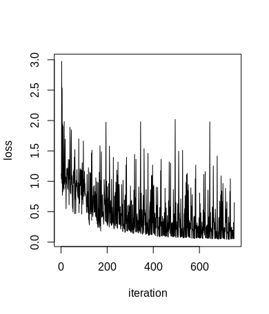
Plotting the loss trajectory, we find that the loss in general decreases with an increasing number of iterations. The trajectory is not smooth, since we see the prediction loss for every individual data point, and some data points are in general more difficult to classify than others. Adapting the parameter values after each individual prediction is not necessarily the best or most efficient scheme to train a neural network (or any model trained via gradient descent), but our make-shift formulation of the neural network and of its loss does not easily allow gradient calculation for accumulated losses (it would incur the writing of a large amount of repetitive code). Still, we can be quite happy to observe that the loss does decrease markedly.
plot(loss_list, type = 'l')
Finally, we can use the trained parameters to generate and visualize predictions (this was not possible with the previous formulation of the neural network, since it directly returned the loss, and not the prediction itself). To this end, we extract the single components of the neural network that return the outputs of the three nodes of the output layer. We embed them into a loop that iterates over all 150 data points and inserts the values returned by the three output nodes into a matrix with three columns (corresponding to the three output nodes and to the three classes) and 150 rows (corresponding to the individual data points).
preds_mat = matrix(nrow = nrow(iris), ncol = 3)

for(j in 1:nrow(iris)){
  in1a = my_iris[j,1]
  in1b = my_iris[j,2]
  in1c = my_iris[j,3]
  in1d = my_iris[j,4]

  a1 = exp((x2a1 * 1/(1+exp(-(x1a1 * in1a + x1b1 * in1b + x1c1 * in1c + x1d1 * in1d + x1e1 * 1))) +
               x2b1 * 1/(1+exp(-(x1a2 * in1a + x1b2 * in1b + x1c2 * in1c + x1d2 * in1d + x1e2 * 1))) +
               x2c1 * 1/(1+exp(-(x1a3 * in1a + x1b3 * in1b + x1c3 * in1c + x1d3 * in1d + x1e3 * 1))) +
               x2d1 * 1)) /
    (exp((x2a1 * 1/(1+exp(-(x1a1 * in1a + x1b1 * in1b + x1c1 * in1c + x1d1 * in1d + x1e1 * 1))) +
            x2b1 * 1/(1+exp(-(x1a2 * in1a + x1b2 * in1b + x1c2 * in1c + x1d2 * in1d + x1e2 * 1))) +
            x2c1 * 1/(1+exp(-(x1a3 * in1a + x1b3 * in1b + x1c3 * in1c + x1d3 * in1d + x1e3 * 1))) +
            x2d1 * 1)) +
       exp((x2a2 * 1/(1+exp(-(x1a1 * in1a + x1b1 * in1b + x1c1 * in1c + x1d1 * in1d + x1e1 * 1))) +
              x2b2 * 1/(1+exp(-(x1a2 * in1a + x1b2 * in1b + x1c2 * in1c + x1d2 * in1d + x1e2 * 1))) +
              x2c2 * 1/(1+exp(-(x1a3 * in1a + x1b3 * in1b + x1c3 * in1c + x1d3 * in1d + x1e3 * 1))) +
              x2d2 * 1)) +
       exp((x2a3 * 1/(1+exp(-(x1a1 * in1a + x1b1 * in1b + x1c1 * in1c + x1d1 * in1d + x1e1 * 1))) +
              x2b3 * 1/(1+exp(-(x1a2 * in1a + x1b2 * in1b + x1c2 * in1c + x1d2 * in1d + x1e2 * 1))) +
              x2c3 * 1/(1+exp(-(x1a3 * in1a + x1b3 * in1b + x1c3 * in1c + x1d3 * in1d + x1e3 * 1))) +
              x2d3 * 1)))

  b1 = exp((x2a2 * 1/(1+exp(-(x1a1 * in1a + x1b1 * in1b + x1c1 * in1c + x1d1 * in1d + x1e1 * 1))) +
               x2b2 * 1/(1+exp(-(x1a2 * in1a + x1b2 * in1b + x1c2 * in1c + x1d2 * in1d + x1e2 * 1))) +
               x2c2 * 1/(1+exp(-(x1a3 * in1a + x1b3 * in1b + x1c3 * in1c + x1d3 * in1d + x1e3 * 1))) +
               x2d2 * 1)) /
    (exp((x2a1 * 1/(1+exp(-(x1a1 * in1a + x1b1 * in1b + x1c1 * in1c + x1d1 * in1d + x1e1 * 1))) +
            x2b1 * 1/(1+exp(-(x1a2 * in1a + x1b2 * in1b + x1c2 * in1c + x1d2 * in1d + x1e2 * 1))) +
            x2c1 * 1/(1+exp(-(x1a3 * in1a + x1b3 * in1b + x1c3 * in1c + x1d3 * in1d + x1e3 * 1))) +
            x2d1 * 1)) +
       exp((x2a2 * 1/(1+exp(-(x1a1 * in1a + x1b1 * in1b + x1c1 * in1c + x1d1 * in1d + x1e1 * 1))) +
              x2b2 * 1/(1+exp(-(x1a2 * in1a + x1b2 * in1b + x1c2 * in1c + x1d2 * in1d + x1e2 * 1))) +
              x2c2 * 1/(1+exp(-(x1a3 * in1a + x1b3 * in1b + x1c3 * in1c + x1d3 * in1d + x1e3 * 1))) +
              x2d2 * 1)) +
       exp((x2a3 * 1/(1+exp(-(x1a1 * in1a + x1b1 * in1b + x1c1 * in1c + x1d1 * in1d + x1e1 * 1))) +
              x2b3 * 1/(1+exp(-(x1a2 * in1a + x1b2 * in1b + x1c2 * in1c + x1d2 * in1d + x1e2 * 1))) +
              x2c3 * 1/(1+exp(-(x1a3 * in1a + x1b3 * in1b + x1c3 * in1c + x1d3 * in1d + x1e3 * 1))) +
              x2d3 * 1)))

  c1 = exp((x2a3 * 1/(1+exp(-(x1a1 * in1a + x1b1 * in1b + x1c1 * in1c + x1d1 * in1d + x1e1 * 1))) +
               x2b3 * 1/(1+exp(-(x1a2 * in1a + x1b2 * in1b + x1c2 * in1c + x1d2 * in1d + x1e2 * 1))) +
               x2c3 * 1/(1+exp(-(x1a3 * in1a + x1b3 * in1b + x1c3 * in1c + x1d3 * in1d + x1e3 * 1))) +
               x2d3 * 1)) /
    (exp((x2a1 * 1/(1+exp(-(x1a1 * in1a + x1b1 * in1b + x1c1 * in1c + x1d1 * in1d + x1e1 * 1))) +
            x2b1 * 1/(1+exp(-(x1a2 * in1a + x1b2 * in1b + x1c2 * in1c + x1d2 * in1d + x1e2 * 1))) +
            x2c1 * 1/(1+exp(-(x1a3 * in1a + x1b3 * in1b + x1c3 * in1c + x1d3 * in1d + x1e3 * 1))) +
            x2d1 * 1)) +
       exp((x2a2 * 1/(1+exp(-(x1a1 * in1a + x1b1 * in1b + x1c1 * in1c + x1d1 * in1d + x1e1 * 1))) +
              x2b2 * 1/(1+exp(-(x1a2 * in1a + x1b2 * in1b + x1c2 * in1c + x1d2 * in1d + x1e2 * 1))) +
              x2c2 * 1/(1+exp(-(x1a3 * in1a + x1b3 * in1b + x1c3 * in1c + x1d3 * in1d + x1e3 * 1))) +
              x2d2 * 1)) +
       exp((x2a3 * 1/(1+exp(-(x1a1 * in1a + x1b1 * in1b + x1c1 * in1c + x1d1 * in1d + x1e1 * 1))) +
              x2b3 * 1/(1+exp(-(x1a2 * in1a + x1b2 * in1b + x1c2 * in1c + x1d2 * in1d + x1e2 * 1))) +
              x2c3 * 1/(1+exp(-(x1a3 * in1a + x1b3 * in1b + x1c3 * in1c + x1d3 * in1d + x1e3 * 1))) +
              x2d3 * 1)))

  preds_mat[j,] = c(a1, b1, c1)
}
This predictions matrix has the same structure as the ground-truth matrix generated above (before model training). This means that we can now directly compare the predicted class indices (positional argument of the greatest output value among the three output nodes in each row of the predictions matrix) with the true class label (positional argument of the "1" in each row of the ground-truth matrix). We will do so by calculating the squared difference between each cell in the ground-truth matrix and each corresponding cell in the predictions matrix.
Instead of going for some complicated visualization, we will simply look at the squared-differences matrix from a bird's eye perspective using the image() function. This simply converts the matrix into tile plots, where each tile corresponds to one matrix cell. The coloration of the tiles then corresponds to the magnitude of values contained in them. In the following plots, red tiles contain a "1", while yellow cells contain a "zero", tiles with different colors contain values larger than zero but less than one.
image((y_mat - preds_mat)**2)
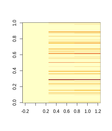
We can easily see that the majority of plant samples were correctly classified by our neural network, since most cells are a pale yellow, indicating a minor difference between the ground truth (zero or one) and the output values of the neural network (values between zero and one). Compare this to the following plot, which shows differences between ground-truth and predictions of an untrained neural network:
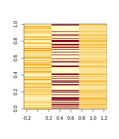
It is easy to see that the training has strongly improved the predictive capability of the neural network.
So, we have successfully completed the task of building and training a neural network from scratch. While it requires a lot of typing effort, and while the written code can look confusing in the beginning, we can trace back all the operations that make the training and the neural network itself work in intricate detail. Only the application of the chain rule to calculate gradients during training is still a bit of a black box, since the deriv function does this job for us. On the other hand, the derivation rules would have to be specified for each calculation step in the neural network individually, so there is not really much of a point to design them manually for demonstrative purpose.