Programming the backpropagation algorithm from scratch
Complex neural networks use the backpropagation algorithm for efficient fitting of their parameters. Since its actual meaning and functioning is often treated somewhat as a given, we are going to take a closer look.
Deep neural networks are complex mathematical graphs, i.e. a sequence of mathematical operations where computations made early on affect all subsequent computations. It is possible to fit parameters in such graphs using the computer's ability for automatic differenciation, and we have in fact done that in an earlier article. Neural networks have the specialty that different parallel parts of the graph are often built upon, i.e. refer to, the same earlier part of the graph. In programming the network for automatic differenciation, this means that the same set of operations must be written multiple times. As the number of layers (i.e. a set of parallel computations) in the graph increases, the number of references to the earliest layers in the graph increases dramatically. The complexity of the resulting equations required for differentiation becomes excessively large, leading to a requirement for large computational resources that can exceed the capabilties of modern computers.
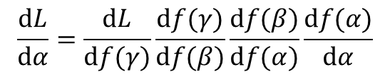
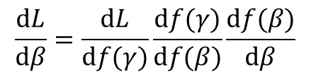
A solution to this difficulty lies in making use of the chain rule. The chain rule states that the partial derivative of the output of a (loss-) function with respect to a specific parameter can be described as the product of a series of partial derivatives, where the first component is the partial derivative of the first intermediate calculation in the graph that incorporates that parameter with respect to that parameter, and the final component is the partial derivative of the output of the graph (i.e., some form of loss value) with respect to the final intermediate calculation in the graph. More concretely, imagine a graph of four computational steps (four "layers", if you will), where parameter alpha is multiplied with some scalar input data point d, and the resulting product f(alpha) (read "function of alpha") is multiplied with parameter beta, and the resulting product is multiplied with parameter gamma, and the scalar output L of the graph is that last product multiplied with parameter delta, then the partial derivative of L with respect to alpha is the following product: d_L / d_alpha = d_L / d_f(gamma) * d_f(gamma) / d_f(beta) * d_f(beta) / d_f(alpha) * d_f(alpha) / d_alpha. Likewise, the partial derivative of L with respect to beta is d_L / d_beta = d_l / d_f(gamma) * d_f(gamma) / d_f(beta) * d_f(beta) / d_beta.
Of course, the example given here is a very simple form of mathematical graph and is not particularly complex, especially since there are not multiple parallel operations that refer to the same preceding parameter, as in neural networks. Still, one can figure out the advantage that the formulation via the chain rule offers: It is possible to actually calculate all intermediate products (f(alpha), ..., f() that are generated within the graph, plus the loss (or the final product) L, i.e. one can obtain an actual numeric value for each product. Then, one can calculate the single partial derivatives listed above by referring to these numeric values, i.e. calculate the partial derivative of a given product (as a symbolic mathematical operation) with respect to the preceding product (a scalar numerical value). Generalizing, one would calculate the partial derivative of any given mathematical operation with respect to the numerical output of a preceding operation that is included in the current operation. Let us take a look at that on another example: Here, we multiply a parameter w with a scalar input x, apply a sequence of three logistic transformations (or sigmoid activations, of the form f(x) = 1 / (1 + exp(-x))), and calculate the squared difference of this "prediction" from some observed value y. We can disaggreagte the series of operations into three shorter sequences: The first multiplies w with x and applies the first logistic transformation, the second applies the second logistic transformation, and the third applies the third logistic transformation and calculates the squared difference from y. beta is d_L / d_beta = d_l / d_f(gamma) * d_f(gamma) / d_f(beta) * d_f(beta) / d_beta.
We can calculate the partial derivative of the output of the squared-difference calculation (i.e., the loss calculation) with respect to w by applying the deriv function to the entire graph of calculations, from the initial multiplication of w with x to the squarring of the difference between y and the prediction.
x = 3.5
w = 2.5
y = 9.5

d = deriv(~ (y - 1 / (1 + exp(-(1 / (1 + exp(-(1 / (1 + exp(-w * x)))))))))**2, 'w')

eval(d)
Or we can calculate scalar outputs for the first two of the three disaggregated terms of the original graph (the so-called "forward pass"), and calculate partial derivatives of their result with respect to their input, which happens to be w for the first term and the respective preceding term for the second and third terms. The three resulting gradients are then multiplied (this is the final step of the so-called "backward pass"), and the product equals the partial derivative calculated above using the entire computational graph.
part1 = 1 / (1 + exp(-w * x))
part2 = 1 / (1 + exp(-part1))

d1 = deriv(~ (y - 1 / (1 + exp(-(part2))))**2, 'part2')
d2 = deriv(~ 1 / (1 + exp(-(part1))), 'part1')
d3 = deriv(~ 1 / (1 + exp(-(w * x))), 'w')

attributes(eval(d1))[[1]] * attributes(eval(d2))[[1]] * attributes(eval(d3))[[1]]
Let us now look at a more applied and more complex example: the classification of plants of the genus Iris according to attributes of their flowers. We have addressed this task several times before, and have even used a neural network, but have not yet applied true back-propagation. Here, we will use the same simple neural network again, which consists of one hidden layer and one output layer. Both the hidden layer and the output layer create three-dimensional representations of the data (have three "nodes"); the dimensionality of the hidden layer is arbitrary, that of the output layer is defined by the number of classes in the data (three species). A sigmoid activation is applied on the sum-products of input variables and parameters in the hidden layer, while a softmax activation is applied on the sum-products of the components of the hidden representation and parameters in the output layer (see details below).While referring to the dimensionality of the intial or of an intermediate representation of the data associated with a given layer, one often speaks about the number of nodes of that layer. The term node is somewhat unclearly defined and can refer to both a partial set of computations in a given layer or to a partial output of that layer.
We first need to do some preparatory work: As always, we standardize the input data along each variable, i.e. we subtract the mean of every variable from the corresponding value of the single data points and divide the differences by the standard deviation of the variable. In the iris data set, we have four numeric variables. The fifth variable giving the class identity is used to set up a matrix of ground-truth values in the form of one-hot-encoded vectors that will be compared to the prediction of the network and will thus be used to calculate its performance loss. Each vector has three elements, two of which have zero value and one which has a value of 1; the identity of the element bearing the "1" is determined by the class at hand.
set.seed(0)

inds = sample(seq(1,nrow(iris),1), nrow(iris), replace = F)
iris = iris[inds,] # bringing the data into random order

my_iris = iris[,1:4]

for(i in 1:4){
  my_iris[,i] = (my_iris[,i] - mean(my_iris[,i])) / sd(my_iris[,i])
}

y_mat = matrix(nrow = nrow(iris), ncol = length(unique(iris$Species)))
y_mat[,] = 0
y_mat[iris$Species == unique(iris$Species)[1],1] = 1
y_mat[iris$Species == unique(iris$Species)[2],2] = 1
y_mat[iris$Species == unique(iris$Species)[3],3] = 1
Next, we initialize the parameters of the neural network by picking a random value from a normal distribution for each. There is one parameter for every connection between the input nodes (four) and the nodes of the hidden representation (three). There is one additional parameter (often referred to as "bias") that is not multiplied with any input and is simply added to the hidden representation; there is one such parameter for each node. We thus end up with fourteen parameters in the first hidden layer of the neural network. Further, both the hidden- and the output representation have three dimensions, and thus there are 3 * 3 + 3 = 12 additional parameters to initialize (again as random draws from the standard normal distribution).
x1a1 = rnorm(1)
x1b1 = rnorm(1)
x1c1 = rnorm(1)
x1d1 = rnorm(1)
x1e1 = rnorm(1)
x1a2 = rnorm(1)
x1b2 = rnorm(1)
x1c2 = rnorm(1)
x1d2 = rnorm(1)
x1e2 = rnorm(1)
x1a3 = rnorm(1)
x1b3 = rnorm(1)
x1c3 = rnorm(1)
x1d3 = rnorm(1)
x1e3 = rnorm(1) # parameters of the hidden layer. Letters a,...,d refer to the input dimensions,
# numbers 1,2,3 refer to the nodes of the hidden layer. 'e' denotes a bias parameter

x2a1 = rnorm(1)
x2b1 = rnorm(1)
x2c1 = rnorm(1)
x2d1 = rnorm(1)
x2a2 = rnorm(1)
x2b2 = rnorm(1)
x2c2 = rnorm(1)
x2d2 = rnorm(1)
x2a3 = rnorm(1)
x2b3 = rnorm(1)
x2c3 = rnorm(1)
x2d3 = rnorm(1) # parameters of the output layer. Letters a,b,c refer to the nodes of the hidden layer,
# number 1,2,3 refer to the nodes of the output layer. 'd' denotes a bias parameter
We now perform the computations of the neural network (the forward pass). First, we select the first sample from our iris data set and multiply the four variables with the corresponding parameters of the first layer that connect the input data to the first node of the hidden layer. We add up the products and then add the bias parameter. Finally, we apply the logistic transformation (or "sigmoid activation") on the sum (1 / (1 + exp(-input))). We repeat these steps for each of the three nodes of the hidden layer.
in1a = my_iris[1,1]
in1b = my_iris[1,2]
in1c = my_iris[1,3]
in1d = my_iris[1,4]

y_1 = y_mat[1,1]
y_2 = y_mat[1,2]
y_3 = y_mat[1,3]

l1_1 = 1/(1+exp(-(x1a1 * in1a + x1b1 * in1b + x1c1 * in1c + x1d1 * in1d + x1e1 * 1)))
l1_2 = 1/(1+exp(-(x1a2 * in1a + x1b2 * in1b + x1c2 * in1c + x1d2 * in1d + x1e2 * 1)))
l1_3 = 1/(1+exp(-(x1a3 * in1a + x1b3 * in1b + x1c3 * in1c + x1d3 * in1d + x1e3 * 1)))
Next, we perform the operations of the output layer: We now multiply each dimension of the hidden representation (corresponding to the nodes of the hidden layer) with each of the three parameters connecting them to the first of the three nodes of the output layer. We sum the three products and add the bias parameter of the first output node. Before we can transform the sum with the categorical-crossentropy function, we need to repeat the operation for both the second and the third node of the output layer, since all three sums are required in that function.
l2_1 = x2a1 * l1_1 + x2b1 * l1_2 + x2c1 * l1_3 + x2d1 * 1
l2_2 = x2a2 * l1_1 + x2b2 * l1_2 + x2c2 * l1_3 + x2d2 * 1
l2_3 = x2a3 * l1_1 + x2b3 * l1_2 + x2c3 * l1_3 + x2d3 * 1
Having computed all sums, we apply the softmax function on each value of the output vector (i.e., the result of the computations in the output layer). The softmax function for a given output value is the exponentiated output value divided by the sum over the entire exponentiated output vector. It ensures that the outputs of the neural network sum to one. The class prediction of the neural network is then the index of the greatest output value in the output vector.
c(exp(l2_1) / (exp(l2_1) + exp(l2_2) + exp(l2_3)),
                    exp(l2_2) / (exp(l2_1) + exp(l2_2) + exp(l2_3)),
                    exp(l2_3) / (exp(l2_1) + exp(l2_2) + exp(l2_3)))

pred = which(c(exp(l2_1) / (exp(l2_1) + exp(l2_2) + exp(l2_3)),
                    exp(l2_2) / (exp(l2_1) + exp(l2_2) + exp(l2_3)),
                    exp(l2_3) / (exp(l2_1) + exp(l2_2) + exp(l2_3))) == max(c(exp(l2_1) / (exp(l2_1) + exp(l2_2) + exp(l2_3)),
                                                                              exp(l2_2) / (exp(l2_1) + exp(l2_2) + exp(l2_3)),
                                                                              exp(l2_3) / (exp(l2_1) + exp(l2_2) + exp(l2_3)))))
# the prediction is the index of the maximum value in the output vector
Now, we calculate the loss incurred from the prediction of the neural network. We compare the output of the neural network, which is a vector of three values that some to one, with the one-hot-encoded vector that gives the true class of the sample at hand. The categorical categorical-crossentropy measures the difference between a true and a predicted distribution, and is calculated in the present case as the negative sum of the product of the one-hot-encoded vector with the logarithm of the prediction vector.
ce = -(y_1 * log(exp(l2_1) / (exp(l2_1) + exp(l2_2) + exp(l2_3))) +
              y_2 * log(exp(l2_2) / (exp(l2_1) + exp(l2_2) + exp(l2_3))) +
              y_3 * log(exp(l2_3) / (exp(l2_1) + exp(l2_2) + exp(l2_3))))
Now, we calculate the partial derivatives of that loss value with respect to the parameters of the neural network, in order to be able to update them later on. Previously, we did this in a simple one-step procedure using the deriv function on the entire graph of computations in the neural net, akin to the first procedure presented for the example above. Now, we calculate a "chain" of partial derivatives: First, we calculate the derivative of the categorical crossentropy wih respect to the output layer before the softmax activation, using the deriv function.
d_ce_l2 = deriv(~ -(y_1 * log(exp(l2_1) / (exp(l2_1) + exp(l2_2) + exp(l2_3))) +
                           y_2 * log(exp(l2_2) / (exp(l2_1) + exp(l2_2) + exp(l2_3))) +
                           y_3 * log(exp(l2_3) / (exp(l2_1) + exp(l2_2) + exp(l2_3)))), c('l2_1','l2_2','l2_3')) # derivative of the
# cross-entropy with respect to the non-activated output of the three nodes of the output layer (returns three derivatives, one for each node)
Next, we calculate the partial derivative of the non-activated output of the output layer with respect to i) the parameters connecting the hidden layer and the output layer and ii) with respect to the (activated) output of the hidden layer. We do this operation separately for each of the three output nodes.
d_l2_1_par = deriv(~ x2a1 * l1_1 + x2b1 * l1_2 + x2c1 * l1_3 + x2d1 * 1, c('x2a1', 'x2b1', 'x2c1', 'x2d1')) # derivative of the non-activated
# output of the first node in the output layer with respect to the parameters connecting the hidden layer to that output node
d_l2_1_l1 = deriv(~ x2a1 * l1_1 + x2b1 * l1_2 + x2c1 * l1_3 + x2d1 * 1, c('l1_1', 'l1_2', 'l1_3')) # derivative of the non-activated
# output of the first node in the output layer with respect to the activated output of the hidden layer

d_l2_2_par = deriv(~ x2a2 * l1_1 + x2b2 * l1_2 + x2c2 * l1_3 + x2d2 * 1, c('x2a2', 'x2b2', 'x2c2', 'x2d2'))
d_l2_2_l1 = deriv(~ x2a2 * l1_1 + x2b2 * l1_2 + x2c2 * l1_3 + x2d2 * 1, c('l1_1', 'l1_2', 'l1_3'))

d_l2_3_par = deriv(~ x2a3 * l1_1 + x2b3 * l1_2 + x2c3 * l1_3 + x2d3 * 1, c('x2a3', 'x2b3', 'x2c3', 'x2d3'))
d_l2_3_l1 = deriv(~ x2a3 * l1_1 + x2b3 * l1_2 + x2c3 * l1_3 + x2d3 * 1, c('l1_1', 'l1_2', 'l1_3'))
Finally, we calculate the derivative of the output of the hidden layer with respect to the parameters connecting the input to the neural network (i.e. the numeric variables of a given iris data point) to the nodes of the hidden layer. Note that we calculate the derivatives of the activated outputs this time, since the sigmoid activation, unlike the softmax one, requires no knowledge about the other nodes of the hidden layer. Again, we perform this operation separately for each of the three nodes of the hidden layer.
d_l1_1_par = deriv(~ 1/(1+exp(-(x1a1 * in1a + x1b1 * in1b + x1c1 * in1c + x1d1 * in1d + x1e1 * 1))), c('x1a1', 'x1b1', 'x1c1', 'x1d1', 'x1e1'))
# derivative of the output of the first node in the hidden layer with respect to the parameters connecting the input data point to that
# hidden node
d_l1_2_par = deriv(~ 1/(1+exp(-(x1a2 * in1a + x1b2 * in1b + x1c2 * in1c + x1d2 * in1d + x1e2 * 1))), c('x1a2', 'x1b2', 'x1c2', 'x1d2', 'x1e2'))
d_l1_3_par = deriv(~ 1/(1+exp(-(x1a3 * in1a + x1b3 * in1b + x1c3 * in1c + x1d3 * in1d + x1e3 * 1))), c('x1a3', 'x1b3', 'x1c3', 'x1d3', 'x1e3'))
Now, we combine the results generated from the above calculations to compute the final gradients of the loss with respect to the parameters of the neural network: We begin with the parameters that connect the hidden layer to the output layer. Since in the forward pass the application of the parameters is followed by the softmax transformation before the loss is calculated, we need to multiply the derivative of the pre-transformed layer output with respect to the layer"s parameters with the derivative of the prediction loss with respect to the pre-transformed layer output. We obtain the derivative of the loss with respect to the parameters of the output layer. We perform this operation separately for each of the three nodes of the output layer, since each node has its own proper set of parameters connecting it to the hidden layer associated with it.
grads_x2_1 = attributes(eval(d_l2_1_par))['gradient'][[1]][1,][c('x2a1', 'x2b1', 'x2c1', 'x2d1')] * attributes(eval(d_ce_l2))['gradient'][[1]][1,]['l2_1']
# loss gradients of the parameters connecting the hidden layer with the first node of the output layer
grads_x2_2 = attributes(eval(d_l2_2_par))['gradient'][[1]][1,][c('x2a2', 'x2b2', 'x2c2', 'x2d2')] * attributes(eval(d_ce_l2))['gradient'][[1]][1,]['l2_2']
grads_x2_3 = attributes(eval(d_l2_3_par))['gradient'][[1]][1,][c('x2a3', 'x2b3', 'x2c3', 'x2d3')] * attributes(eval(d_ce_l2))['gradient'][[1]][1,]['l2_3']
Next, we calculate the gradient of the loss with respect to the parameters connecting the input to the neural network - the four-dimensional data point - to the three nodes of the hidden layer: We multiply the derivatives of the non-activated output of a given node of the hidden layer with respect to the parameters connecting the input and that non-activated output with the derivatives of the non-activated output of the final layer with respect to the activated outputs of the hidden layer, summed over all three nodes of the output layer. It is necessary to multiply with the sum here, as one node in the hidden layer is connected to all three nodes in the output layer, and thus a parameter affecting that hidden node also indirectly affects all three output nodes. The operation is performed for each node in the hidden layer separately, and we obtain the gradient of the loss with respect to all the weights connecting the input layer and the hidden layer as the end result.
grads_x1_1 = attributes(eval(d_l1_1_par))['gradient'][[1]][1,][c('x1a1', 'x1b1', 'x1c1', 'x1d1', 'x1e1')] *
  (attributes(eval(d_l2_1_l1))['gradient'][[1]][1,]['l1_1'] * attributes(eval(d_ce_l2))['gradient'][[1]][1,]['l2_1'] +
  attributes(eval(d_l2_2_l1))['gradient'][[1]][1,]['l1_1'] * attributes(eval(d_ce_l2))['gradient'][[1]][1,]['l2_2'] +
  attributes(eval(d_l2_3_l1))['gradient'][[1]][1,]['l1_1'] * attributes(eval(d_ce_l2))['gradient'][[1]][1,]['l2_3']) # loss gradients of the
# parameters connecting the input data point with the first node of the hidden layer

grads_x1_2 = attributes(eval(d_l1_2_par))['gradient'][[1]][1,][c('x1a2', 'x1b2', 'x1c2', 'x1d2', 'x1e2')] *
  (attributes(eval(d_l2_1_l1))['gradient'][[1]][1,]['l1_2'] * attributes(eval(d_ce_l2))['gradient'][[1]][1,]['l2_1'] +
  attributes(eval(d_l2_2_l1))['gradient'][[1]][1,]['l1_2'] * attributes(eval(d_ce_l2))['gradient'][[1]][1,]['l2_2'] +
  attributes(eval(d_l2_3_l1))['gradient'][[1]][1,]['l1_2'] * attributes(eval(d_ce_l2))['gradient'][[1]][1,]['l2_3'])

grads_x1_3 = attributes(eval(d_l1_3_par))['gradient'][[1]][1,][c('x1a3', 'x1b3', 'x1c3', 'x1d3', 'x1e3')] *
  (attributes(eval(d_l2_1_l1))['gradient'][[1]][1,]['l1_3'] * attributes(eval(d_ce_l2))['gradient'][[1]][1,]['l2_1'] +
  attributes(eval(d_l2_2_l1))['gradient'][[1]][1,]['l1_3'] * attributes(eval(d_ce_l2))['gradient'][[1]][1,]['l2_2'] +
  attributes(eval(d_l2_3_l1))['gradient'][[1]][1,]['l1_3'] * attributes(eval(d_ce_l2))['gradient'][[1]][1,]['l2_3'])
We finally use the gradients just obtained to adjust the parameters of the neural network: We subtract the gradient multiplied with a fixed learning rate - the step-width of the parameter updates - from the original parameter value. By updating the parameters several times, they should gradually converge towards optimal values, i.e. values that reduce the prediction loss as far as possible (that does not necessarily imply that the model is then the best it can be, as it needs to be tested for generalizing capability also).
all_grads = c(grads_x1_1, grads_x1_2, grads_x1_3, grads_x2_1, grads_x2_2, grads_x2_3) # combining all loss gradients into one vector

lr = 1e-1 # learning rate

unlist(lapply(seq(1, length(all_grads)), function(i){
  eval(parse(text = paste0(names(all_grads)[i], " = ", names(all_grads)[i], " - lr * all_grads['", names(all_grads)[i], "']")))
  eval(parse(text = paste0("assign('", names(all_grads)[i], "', ", names(all_grads)[i], ", .GlobalEnv)")))
})) # using a loop to update all parameters of the neural network
We can now insert the sequence of procedures - computing the prediction of the neural network and all of the intermediate results, calculating the partial derivatives of the prediction loss or of the intermediate results of the network with respect to its parameters of preceding results, and using the chain rule to obtain the gradients of the loss with respect to the network parameters from these derivatives - into a loop that goes over all data points in the iris data set. In our simplified example, the parameters are updated after the prediction of each single data point; in applied usage, one would rather accumulate the loss incurred from predictions on several data points before updating the parameters. Anyhow, we also embed this inner loop into an outer loop that iterates over a number of steps and repeats the process of prediction-making and parameter updates over all 150 data points at every step. This number of steps could be optimized by tracing the improvement in predictive skill of the neural network; however, in the present illustrative example, we forego this procedure.
for(k in 1:50){ # iterating over 50 steps
  for(j in 1:nrow(my_iris)){ # iterating over the 150 data points in the data set
    in1a = my_iris[j,1]
    in1b = my_iris[j,2]
    in1c = my_iris[j,3]
    in1d = my_iris[j,4]

    y_1 = y_mat[j,1]
    y_2 = y_mat[j,2]
    y_3 = y_mat[j,3]

    l1_1 = 1/(1+exp(-(x1a1 * in1a + x1b1 * in1b + x1c1 * in1c + x1d1 * in1d + x1e1 * 1)))
    l1_2 = 1/(1+exp(-(x1a2 * in1a + x1b2 * in1b + x1c2 * in1c + x1d2 * in1d + x1e2 * 1)))
    l1_3 = 1/(1+exp(-(x1a3 * in1a + x1b3 * in1b + x1c3 * in1c + x1d3 * in1d + x1e3 * 1)))

    l2_1 = x2a1 * l1_1 + x2b1 * l1_2 + x2c1 * l1_3 + x2d1 * 1
    l2_2 = x2a2 * l1_1 + x2b2 * l1_2 + x2c2 * l1_3 + x2d2 * 1
    l2_3 = x2a3 * l1_1 + x2b3 * l1_2 + x2c3 * l1_3 + x2d3 * 1

    pred = which(c(exp(l2_1) / (exp(l2_1) + exp(l2_2) + exp(l2_3)),
                    exp(l2_2) / (exp(l2_1) + exp(l2_2) + exp(l2_3)),
                    exp(l2_3) / (exp(l2_1) + exp(l2_2) + exp(l2_3))) == max(c(exp(l2_1) / (exp(l2_1) + exp(l2_2) + exp(l2_3)),
                                                                              exp(l2_2) / (exp(l2_1) + exp(l2_2) + exp(l2_3)),
                                                                              exp(l2_3) / (exp(l2_1) + exp(l2_2) + exp(l2_3)))))

    ce = -(y_1 * log(exp(l2_1) / (exp(l2_1) + exp(l2_2) + exp(l2_3))) +
              y_2 * log(exp(l2_2) / (exp(l2_1) + exp(l2_2) + exp(l2_3))) +
              y_3 * log(exp(l2_3) / (exp(l2_1) + exp(l2_2) + exp(l2_3))))

    print(ce) # printing the loss

    d_ce_l2 = deriv(~ -(y_1 * log(exp(l2_1) / (exp(l2_1) + exp(l2_2) + exp(l2_3))) +
                           y_2 * log(exp(l2_2) / (exp(l2_1) + exp(l2_2) + exp(l2_3))) +
                           y_3 * log(exp(l2_3) / (exp(l2_1) + exp(l2_2) + exp(l2_3)))), c('l2_1','l2_2','l2_3'))

    d_l2_1_par = deriv(~ x2a1 * l1_1 + x2b1 * l1_2 + x2c1 * l1_3 + x2d1 * 1, c('x2a1', 'x2b1', 'x2c1', 'x2d1'))
    d_l2_1_l1 = deriv(~ x2a1 * l1_1 + x2b1 * l1_2 + x2c1 * l1_3 + x2d1 * 1, c('l1_1', 'l1_2', 'l1_3'))

    d_l2_2_par = deriv(~ x2a2 * l1_1 + x2b2 * l1_2 + x2c2 * l1_3 + x2d2 * 1, c('x2a2', 'x2b2', 'x2c2', 'x2d2'))
    d_l2_2_l1 = deriv(~ x2a2 * l1_1 + x2b2 * l1_2 + x2c2 * l1_3 + x2d2 * 1, c('l1_1', 'l1_2', 'l1_3'))

    d_l2_3_par = deriv(~ x2a3 * l1_1 + x2b3 * l1_2 + x2c3 * l1_3 + x2d3 * 1, c('x2a3', 'x2b3', 'x2c3', 'x2d3'))
    d_l2_3_l1 = deriv(~ x2a3 * l1_1 + x2b3 * l1_2 + x2c3 * l1_3 + x2d3 * 1, c('l1_1', 'l1_2', 'l1_3'))

    d_l1_1_par = deriv(~ 1/(1+exp(-(x1a1 * in1a + x1b1 * in1b + x1c1 * in1c + x1d1 * in1d + x1e1 * 1))), c('x1a1', 'x1b1', 'x1c1', 'x1d1', 'x1e1'))
    d_l1_2_par = deriv(~ 1/(1+exp(-(x1a2 * in1a + x1b2 * in1b + x1c2 * in1c + x1d2 * in1d + x1e2 * 1))), c('x1a2', 'x1b2', 'x1c2', 'x1d2', 'x1e2'))
    d_l1_3_par = deriv(~ 1/(1+exp(-(x1a3 * in1a + x1b3 * in1b + x1c3 * in1c + x1d3 * in1d + x1e3 * 1))), c('x1a3', 'x1b3', 'x1c3', 'x1d3', 'x1e3'))

    grads_x2_1 = attributes(eval(d_l2_1_par))['gradient'][[1]][1,][c('x2a1', 'x2b1', 'x2c1', 'x2d1')] * attributes(eval(d_ce_l2))['gradient'][[1]][1,]['l2_1']
    grads_x2_2 = attributes(eval(d_l2_2_par))['gradient'][[1]][1,][c('x2a2', 'x2b2', 'x2c2', 'x2d2')] * attributes(eval(d_ce_l2))['gradient'][[1]][1,]['l2_2']
    grads_x2_3 = attributes(eval(d_l2_3_par))['gradient'][[1]][1,][c('x2a3', 'x2b3', 'x2c3', 'x2d3')] * attributes(eval(d_ce_l2))['gradient'][[1]][1,]['l2_3']

    grads_x1_1 = attributes(eval(d_l1_1_par))['gradient'][[1]][1,][c('x1a1', 'x1b1', 'x1c1', 'x1d1', 'x1e1')] *
      (attributes(eval(d_l2_1_l1))['gradient'][[1]][1,]['l1_1'] * attributes(eval(d_ce_l2))['gradient'][[1]][1,]['l2_1'] +
      attributes(eval(d_l2_2_l1))['gradient'][[1]][1,]['l1_1'] * attributes(eval(d_ce_l2))['gradient'][[1]][1,]['l2_2'] +
      attributes(eval(d_l2_3_l1))['gradient'][[1]][1,]['l1_1'] * attributes(eval(d_ce_l2))['gradient'][[1]][1,]['l2_3'])

    grads_x1_2 = attributes(eval(d_l1_2_par))['gradient'][[1]][1,][c('x1a2', 'x1b2', 'x1c2', 'x1d2', 'x1e2')] *
      (attributes(eval(d_l2_1_l1))['gradient'][[1]][1,]['l1_2'] * attributes(eval(d_ce_l2))['gradient'][[1]][1,]['l2_1'] +
      attributes(eval(d_l2_2_l1))['gradient'][[1]][1,]['l1_2'] * attributes(eval(d_ce_l2))['gradient'][[1]][1,]['l2_2'] +
      attributes(eval(d_l2_3_l1))['gradient'][[1]][1,]['l1_2'] * attributes(eval(d_ce_l2))['gradient'][[1]][1,]['l2_3'])

    grads_x1_3 = attributes(eval(d_l1_3_par))['gradient'][[1]][1,][c('x1a3', 'x1b3', 'x1c3', 'x1d3', 'x1e3')] *
      (attributes(eval(d_l2_1_l1))['gradient'][[1]][1,]['l1_3'] * attributes(eval(d_ce_l2))['gradient'][[1]][1,]['l2_1'] +
      attributes(eval(d_l2_2_l1))['gradient'][[1]][1,]['l1_3'] * attributes(eval(d_ce_l2))['gradient'][[1]][1,]['l2_2'] +
      attributes(eval(d_l2_3_l1))['gradient'][[1]][1,]['l1_3'] * attributes(eval(d_ce_l2))['gradient'][[1]][1,]['l2_3'])

    all_grads = c(grads_x1_1, grads_x1_2, grads_x1_3, grads_x2_1, grads_x2_2, grads_x2_3)

    lr = 1e-1

    unlist(lapply(seq(1, length(all_grads)), function(i){
      eval(parse(text = paste0(names(all_grads)[i], " = ", names(all_grads)[i], " - lr * all_grads['", names(all_grads)[i], "']")))
      eval(parse(text = paste0("assign('", names(all_grads)[i], "', ", names(all_grads)[i], ", .GlobalEnv)")))
    }))
  }
}
In the present example, we made two simplifcations in the initialization and updating of the parameters of the neural network: I) We picked the start values of the parameters from a simple normal distribution. Research into the optimal initialiation of neural networks has, however, shown that constraining the range of initial values with respect to the dimensionality of data before and after having passed a particular layer can improve the model"s optimization. The distribution of values from which initial parameter values are picked thus depends on the layer set-up of the neural network; it is referred to as the Glorot-uniform distribution (Glorot & Bengio, 2010). II) We implemented a very simple optimization scheme that simply updates parameter values based on the gradients computed from the loss in a given iteration and with a fixed learning rate. A great deal of research has been exerted onto the development of sophisticated optimization algorithms that trace the development of the loss and the parameter values over optimization steps, and adjust the learning rate and additional components of the parameter update in order to enable a faster and more reliable convergence to the loss minimum, i.e. to the set of parameters that allows for the greatest predictive capability of the model. As of today, the state-of-the-art optimizer for (deep) neural networks is the Adam optimizer (Kingma & Ba, 2017). In the example above, we have omitted the implementation of sampling from the Glorot-uniform distribution and of updating parameter values with the Adam algorithm, but if you are interested in an implementation, look here for the adjusted code.
Note that in the present example, the recording and plotting of loss values and predictions was omitted for simplicity"s sake. See the article on building a neural network from scratch to see how this is done. You can simply add the correspondig lines to the code above.
Glorot, X. & Bengio, J. (2010): Understanding the difficulty of training deep feedforward neural networks. Proceedings of the Thirteenth International Conference on Artificial Intelligence and Statistics (PMLR) 9: 249-256
Kingma, D. P. & Ba, J. (2017): Adam: A method for stochastic optimization. arXiv:1412.6980