Ex Data, Scientia

Working with expressions in R

Working with expressions in R can be a powerful tool when the application of loops or functions is not useful. Here, we will explore the usage of expressions in an easy-to-follow example.

Equal program actions that need to be applied to a large body of object instances usually rely on loops to apply the action iteratively on each instance. However, there are cases where such an approach does not yield fruitful results. Take, for example, the case where one has generated a ggplot object and would like to add a large number of layers. An example application of this case could be to demonstrate the different fits of a simple linear regression model to a set of data when utilizing different model-parameter values. Instinctively, one would generate a baseline plot object containing a scatter-plot layer for the observed data, and would then use a loop to iteratively add line-plot layers, one for each set of parameters.

intc = 3.0001
slps = seq(0,1.5,length.out = 20)

library('tidyverse')
p = ggplot() +
  geom_point(aes(anscombe$x1, anscombe$y1))

for(i in 1:15){
  p = p + geom_line(aes(anscombe$x1, intc + anscombe$x1 * slps[i]), color = rainbow(15)[i])
}

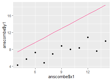
Then, one would enter the name of the plot object into the console, and expect to see a scatter plot of the original data, overlaid by one regression line for each differently parameterized model.

p

Now comes the moment of surprise: We see only the scatter plot and one single regression line. Where have the other lines gone? The answer lies in the fact that ggplot works in a "lazy" fashion by interpreting the commands given in the loop as additions to an overall expression, and not by actually executing the command as soon as it is called in the loop (this also explains why the loop runs relatively fast). The finished expression is then evaluated after the loop has completed the last iteration. Now, the ggplot expression contains as many line-type layers as there were iterations in the loop (i.e., as many layers as there are different parameter sets), but every layer refers to the i-th subset of the data. As i (or any other index name we have used) is now equal to the number of iterations, we only get to see the regression line for the last set of parameter values when calling the plot object (which equals the evaluation of the ggplot expression). In fact, the same line is plotted i times; since these lines all lie on top of each-other, we get the impression of a single line being drawn.

How can we circumvent this problem? Now that we now that we can basically assemble an expression before executing it, we can create a set of expressions that will each access the proper subset of data to be plotted, rather than all accessing the same subset. We set up an empty list-type vector, which should have the same length as the number of parameterization schemes we would like to plot. Then we build a loop which fills this list with expressions (i.e. character strings) for the single line-plot layers. We use the paste0 function to insert the proper index into each expression, so that they do not all refer to i, but instead to the proper index value.

xprs = vector('list', length = 15)

for(i in 1:15){
  xprs[[i]] = paste0("geom_line(aes(anscombe$x1, intc + anscombe$x1 * ",slps[i],"), color = '",rainbow(15)[i],"')")
}

After running the loop, we take the filled list and concatenate the single expressions to one big expression. We again use the paste0 expression for this, and provide a "+" to the collapse argument, which defines how the list components should be connected. By using the plus symbol, the compiled expression will evaluate to a properconcatenation of ggplot layers (these are always concatenated with the plus symbol).

xprs = paste0(xprs, collapse = ' + ')

Finally, we require an expression for the initializing ggplot command and for the scatter-plot layer that will show the observed data. We define this expression, and connect it with our previously generated expression containing the line-plot layers. Note that the initial expression should end with a plus symbol in order to achieve a proper concatenation with the lineplots expression (i.e. a concatenation that, when expressed, yields a proper ggplot command).

base_xpr = "ggplot() +
  geom_point(aes(anscombe$x1, anscombe$y1)) + "
  
plot_xpr = paste0(base_xpr, xprs)

Now, we use the parse command to turn the character string into a proper expression-type object. Finally, we use the eval command to evaluate the expression.

plot_xpr = parse(text = plot_xpr)

eval(plot_xpr)

We find that we achieve a proper plot now, with one line for each parameterization of the regression model, as originally intended.

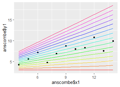
This is just one example of the many possibilities that programming with expressions offers. They are particularly useful to use with loops, when otherwise one would have to invest a lot of tedious writing work to generate the desired command.