Ex Data, Scientia

Data Investigation with Kernel-Density Estimation

Kernel-density estimation (KDE) is a methodology to detect patterns in (often multi-variate) data without imposing the constraint of pre-defining the existence of a certain number of clusters. Basically speaking, KDE tries to detect "commonness" in the data.

It works by calculating the probability density for every data-point (that is, a vector with as many dimensions as there are variables) on the probability-density function defined defined by every data-point (except itself) and by the multivariate standard deviation over the whole data set (the covariance matrix).

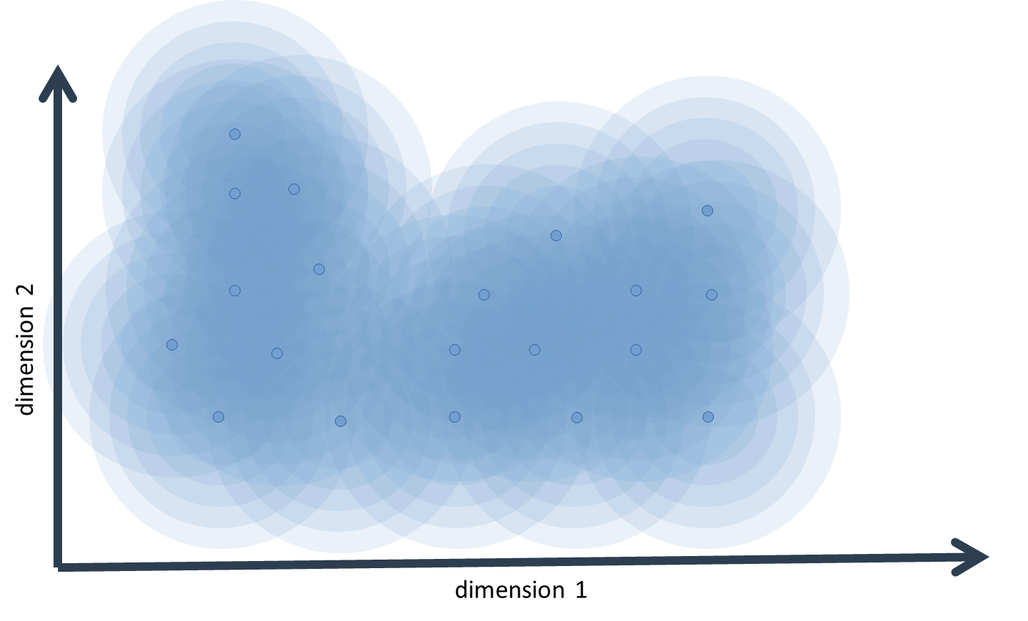
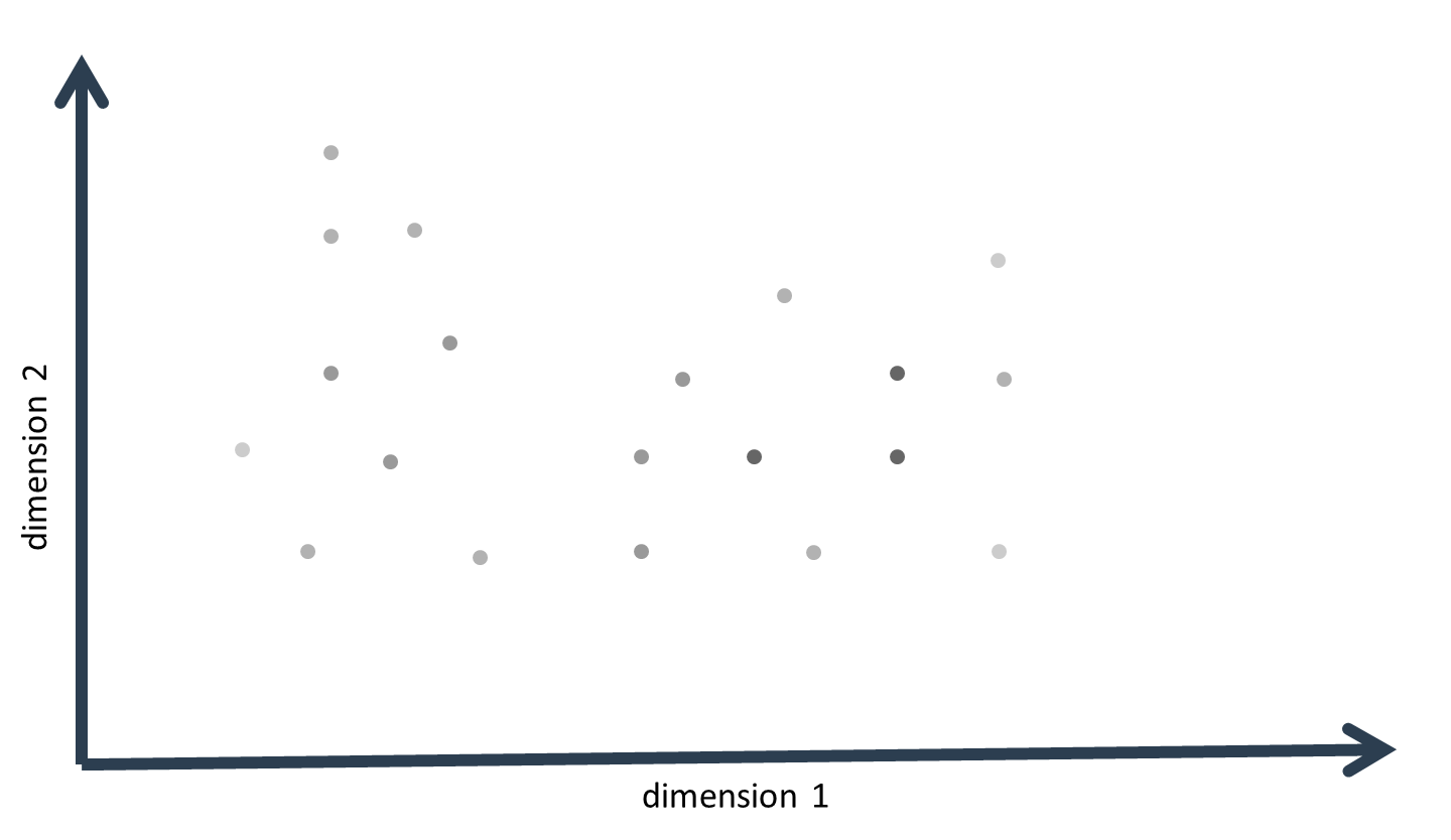
The probability-density values obtained for each data-point (the number equals the total number of data-points minus one) are then summed up. When plotting these so-called kernel-density estimates as a color index on the multivariate data, it becomes obvious that data-points that lie in a large neighborhood of data-points have a large kernel-density estimate, while points that lie more separated from the rest have a low kernel-density estimate. A kernel, in this sense, is then a center of gravity around which data-points cluster.

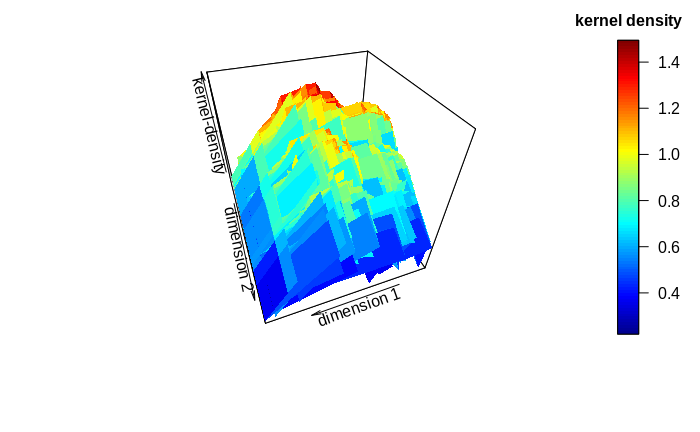
KDE is of limited value for true cluster identification and description. The number of clusters (or kernels) may be approximated from graphical inspection of the sums of the kernel-density estimates in relation to the data: There will often be a dominant cluster, but side clusters may also become apparent if kernel densities do not decrease continuously from the dominating kernel. This may become particularly apparent by generating inference or surface (3D) plots of the kernel sums. Also, the approximate cluster centers represent good starting values for true cluster identification algorithms like K-means or expectation-maximization (EM).

One important factor in cluster detection lies in the so-called bandwidth of the probability distributions: The standard deviation describing a probability distribution may be multiplied with a scalar so to flatten or pronounce the curve of the probability distribution. Depending on the bandwidth, data-points may have a lower or higher probability-density value on the distribution. Thus, clusters may appear or disappear according to bandwidth. It appears recommendable to test the kernel-density estimation with various bandwidths to discover persistent patterns. When the number of clusters can be approximated to lie within a certain range, the persistence check of a true cluster-identification algorithm (e.g. EM) may be employed to further define the true number of clusters.

The application of KDE to univariate data results in the approximation of a smoother, a common graphical data-inspection tool that is e.g. part of the ggplot2 package in R. Here, the characterization of the standard deviation used for the defining the probability-density functions of the singular data-points has a large impact on the degree of “simplification”, or smoothing, of the data.

KDE can be implemented in Python as follows:

"""
import the required packages
"""
import numpy as np
import pandas as pd
import copy
import matplotlib.pyplot as plt
from scipy.stats import *
from sklearn import datasets

"""
load and stadardize the data (here: the iris dataset provided by the scikit-learn package)
"""
iris = datasets.load_iris()['data']

for i in range(np.shape(iris)[1]):
    iris[:,i] = (iris[:,i] - np.mean(iris[:,i])) / np.std(iris[:,i])

"""
set a band width (that is multiplied with the variance-covariance matrix)
"""    
bndwdth = 0.9

"""
set up the variance-covariance matrix, the n-dimensinal analogue the standard deviation used in the 
1-dimensional (univariate) case
"""
covmat = np.cov(np.transpose(iris))
 
"""
set up an empty array with n(rows) = n(datapoints) and n(columns) = n(datapoints).
Fill the array with the value of the probability-density function for datapoint j
for the distribution defined by datapoint i
"""    
prob_densts = np.zeros([np.shape(iris)[0], np.shape(iris)[0]])   
for i in range(np.shape(iris)[0]):
    distr = multivariate_normal(iris[i,:], bndwdth * covmat)
    for j in range(np.shape(iris)[0]):
        prob_densts[i,j] = distr.pdf(iris[j,:])
        print([i,j])

"""
sum the probability-density values over all datapoints for each datapoint (these are
the kernel-density estimates)
"""        
kernel_sums = np.zeros([np.shape(iris)[0]])
for i in range(np.shape(iris)[0]):
    kernel_sums[i] = np.sum(prob_densts[i,:])

"""
plot the data (different combinations of variables) and the kernel-density estimates
"""
plt.scatter(iris[:,0], iris[:,1], c = kernel_sums)
            
plt.scatter(iris[:,1], iris[:,2], c = kernel_sums)

plt.scatter(iris[:,0], iris[:,2], c = kernel_sums)