Ex Data, Scientia
Home
Contact
Hierarchical clustering
Hierarchical clustering is an attractive method for assigning data to multiple clusters simultaneously, and thereby overcomes constraints posed by more traditional approaches.
In previous articles, we have discussed traditional clustering methods like K-means clustering and the expectation-maximization algorithm. These procedures assign each data point in a data set to one particular cluster, and the cluster algorithms converge once cluster assignment changes only minimally. They do not, however, consider the possibility that data points could belong to several clusters, i.e. they are unable to generate over-lapping or nested clusters.
Such an approach - a Hierarchical clustering, may however be more appropriate than the simpler approaches named, especially when dealing with data taken in a natural environment (field data), where certain groups of data may be more similar to each other than to other groups, and where differences in certain variables may be greater than in others. Here, we are going to look at a manual implementation of a hierarchical-clustering algorithm in R, which is applied on the well-known iris data set. This data set contains data on four variables of 150 individual plants belonging to three species of the genus Iris. For our propose of clustering, we assume that we do not know the number of species nor which individual belongs to which species.
We start by standardizing the iris data, that means, for every variable we subtract its mean from the individual values and then divide the difference by its standard deviation. This way, each variable receives a mean of zero and a standard deviation of one, and different magnitudes of the different variables no longer affect the clustering calculations disproportionally.
library('tidyverse')
library('ggforce')

my_iris = iris
for(i in 1:4){
  my_iris[,i] = (my_iris[,i] - mean(my_iris[,i])) / sd(iris[,i])
}
my_iris = my_iris[,1:4]

inds_arr = array(dim = c(150,150)) # setting up matrix to fill with row indices
Next, we pick the first row of the standardized iris data. We then determine the data point that is nearest to our current data point, by calculating the differences, summed over the four variables, between the current pick and all 149 other data points. The closest data point is then the one for which the summed difference is smallest. In case there are two or more data points that share this condition, we simply pick the first one. This is, arguably, a naive constraint; however, from my experience, the situation occurs rather rarely. (An alternative would be to pick a random data point of those that fulfill the "closest-neighbour" condition, and running the overall clustering algorithm for several times.) Continuing with this closest data point, we repeat the procedure of finding the closest data point. We explicitly do not exclude the initial pick, so in theory, the first and the second data point could be their mutual closest "neighbours". In practice, however, this is rather rarely the case. We now continue this search for the closest data point for each following data point, until we return to a data point that we have encountered before. Then we stop this particular part of the clustering algorithm, and we assume that we have found our first cluster, which mathematically represents an undirected graph. We then return to the beginning and pick the second row of the standardized iris data. We repeat the procedure of searching for the closest data point, and of creating a graph of closest data points, which is finished once a data point has been encountered twice. We have then found our next cluster. This may be identical to the first cluster, completely new, over-lapping with the first cluster, or be nested within the first cluster. We repeat the procedure of generating a cluster for each of the following 148 data points.
for(h in 1:150){ # looping over all rows / data points
  ind = h
  i = 1

  inds_arr[h,i] = ind # the index of the current row is added to the index matrix

  while(sum(inds_arr[h,]==ind, na.rm = T) < 2){ # as long as one row index is not encountered twice, the search for nearest neighbours continues
    if(exists('ind_new')){
      ind = ind_new # from the second iteration of the inner loop onwards, the row index is updated
    }

    ind_new = which(rowSums(sapply(seq(1,4,1), function(x){abs(my_iris[ind,x] - my_iris[,x])}))[-ind] ==
                        min(rowSums(sapply(seq(1,4,1), function(x){abs(my_iris[ind,x] - my_iris[,x])}))[-ind])) # returns the row index of the closest data point

    ind_new = ind_new[is.na(ind_new)==F]
    ind_new = ind_new[1] # if there are two or more closest data points, only the first one is selected
    ind_new[ind_new >= ind] = ind_new[ind_new >= ind]+1 # if the found data point has a row index that is higher than the current one, a 1 must be added, since the current row index is excluded from the search for the closest data point (to avoid finding "itself")

    i = i+1
    inds_arr[h,i] = ind_new[1] # the index of the closest data point is added to the array
  }
  rm(ind_new)
}
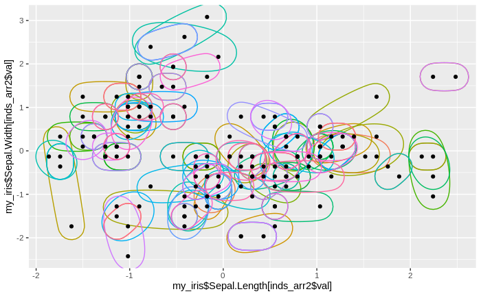
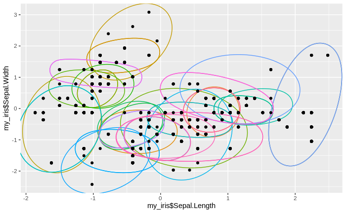
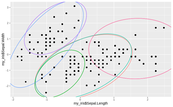
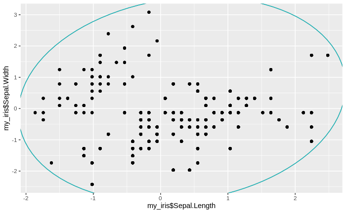
After some tidying of the data, including removing redundant clusters, we can plot the (standardized) data together with the clusters. We note that we have a lot of small clusters, sometimes with just one or two data points in one cluster. We also find that there are many over-lapping and nested clusters, but we also see some clear separations between groups of clusters.
inds_arr = t(inds_arr) # data tidying and re-formatting
inds_arr = as.data.frame(inds_arr)
inds_arr$c_ind = seq(1,nrow(inds_arr),1)

inds_arr2 = inds_arr%>%gather(-c_ind, key = 'rowind', value = 'val')
inds_arr2 = drop_na(inds_arr2)

ggplot() +
  geom_mark_ellipse(aes(my_iris$Sepal.Length[inds_arr2$val], my_iris$Sepal.Width[inds_arr2$val], color = inds_arr2$rowind), show.legend = F) +
  geom_point(aes(my_iris$Sepal.Length, my_iris$Sepal.Width))
Now, we calculate the mean value for each cluster and each variable. We use the standardized values for mean calculation, as opposed to the original values. Furthermore, we calculate the absolute difference between each (standardized) data point and the corresponding cluster means, and sum these differences over the four variables. Note that the standardized iris data set is expanded for this purpose, since several data points are part of multiple clusters, so correspond to several different cluster means. We then sum these summed differences over all data in every cluster, and then calculate and record the median of these sums over all clusters. Naturally, with so many clusters and with relatively few data points in each cluster, the sums of differences will be fairly low. Also, we record the number of clusters (in this case, it matches the number of data points, but this is just a coincidence).
my_iris$val = seq(1,nrow(my_iris),1)
my_iris = full_join(my_iris, inds_arr2%>%select(-c_ind), by = 'val') # combining the cluster indices with the original "iris" data
my_iris = my_iris%>%group_by(rowind)%>%mutate(mn_seplen = mean(Sepal.Length), mn_sepwdt = mean(Sepal.Width), mn_petlen = mean(Petal.Length), mn_petwdt = mean(Petal.Width)) # calculating multivariate means of the "iris" variables, one for each cluster

mn_diff = my_iris%>%mutate(sm_diff = sum(abs(Sepal.Length-mn_seplen) + abs(Sepal.Width-mn_sepwdt) + abs(Petal.Length-mn_petlen) + abs(Petal.Width-mn_petwdt)))%>%group_by(rowind)%>%summarize(sm_diff = sum(sm_diff))%>%ungroup()%>%summarize(median(sm_diff)) # calculating the sum of differences of cluster means to "iris" data for each cluster, then determining the median of these over clusters

n_clusts = length(unique(inds_arr2$rowind)) # determining the number of clusters found
We now standardize the means for each variable and cluster, and use these values to repeat the clustering algorithm described above. Effectively, we now "cluster the clusters". The procedure works exactly as before: For each data point, we determine the closest "neighbouring" data point, and create a graph of data points that are all the closest neighbour to their respective predecessor, until one data point is encountered for a second time. Then, a cluster has been found. This procedure is repeated for every data point. In the end, we have assigned each cluster mean from the first round of the clustering algorithm to a new cluster.
my_subs = distinct(my_iris[,c(7:10)])
my_subs = as.data.frame(my_subs)

for(i in 1:4){
  my_subs[,i+4] = (my_subs[,i] - mean(my_subs[,i])) / sd(my_subs[,i]) # standardizing the cluster means
}

inds_arr = array(dim = c(nrow(my_subs),nrow(my_subs)))

for(h in 1:nrow(my_subs)){ # repeating the clustering procedures for the standardized cluster means from the previous iteration
  ind = h
  i = 1
  inds_arr[h,i] = ind
  while(sum(inds_arr[h,]==ind, na.rm = T) < 2){
    if(exists('ind_new')){
      ind = ind_new
    }
    ind_new = which(rowSums(sapply(seq(5,8,1), function(x){abs(my_subs[ind,x] - my_subs[,x])}))[-ind] ==
                       min(rowSums(sapply(seq(5,8,1), function(x){abs(my_subs[ind,x] - my_subs[,x])}))[-ind]))
    ind_new = ind_new[is.na(ind_new)==F]
    ind_new = ind_new[1]
    ind_new[ind_new >= ind] = ind_new[ind_new >= ind]+1
    i = i+1
    inds_arr[h,i] = ind_new[1]
  }
  rm(ind_new)
}

inds_arr = t(inds_arr)
inds_arr = as.data.frame(inds_arr)
inds_arr$c_ind = seq(1,nrow(inds_arr),1)

inds_arr2 = inds_arr%>%gather(-c_ind, key = 'rowind', value = 'val')
inds_arr2 = drop_na(inds_arr2)

my_subs$val = seq(1,nrow(my_subs),1)
my_subs = full_join(my_subs, inds_arr2%>%select(-c_ind), by = 'val')
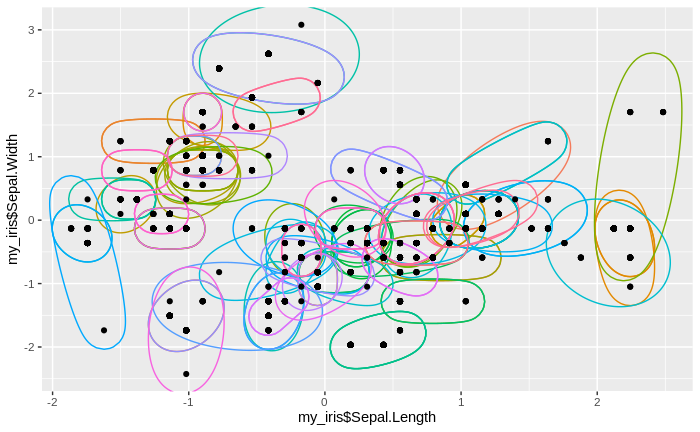
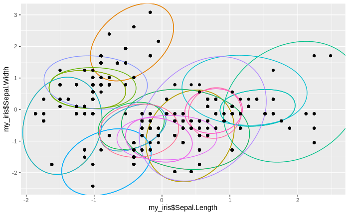
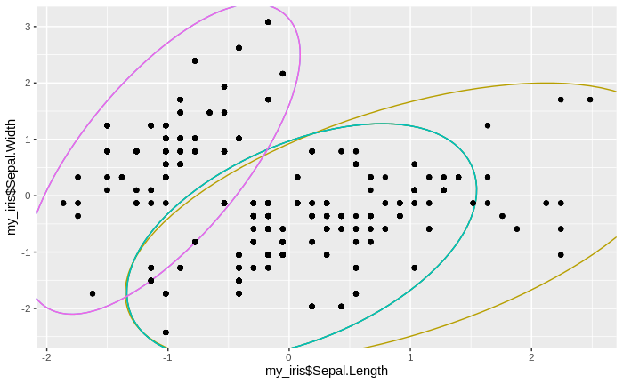
After merging the old cluster means and their new cluster assignments with the original data, we can now plot the new clusters together with the iris data. We do not plot the cluster means, since we are mostly interested in the assignment of the original data to clusters. We find that we now have fewer clusters, with more data per cluster than before.
my_iris = full_join(my_iris, my_subs, by = c("mn_seplen", "mn_sepwdt", "mn_petlen", "mn_petwdt"))

ggplot() +
  geom_mark_ellipse(aes(my_iris$Sepal.Length, my_iris$Sepal.Width, color = my_iris$rowind.y), show.legend = F) +
  geom_point(aes(my_iris$Sepal.Length, my_iris$Sepal.Width))
Again, we record the number of clusters. We also calculate new multivariate cluster means, that is, we calculate one multivariate mean over all original cluster means for every "second-generation" cluster (every cluster obtained in the second round of the clustering algorithm). For these new cluster means, we again calculate the absolute difference to the original (standardized) data, sum these differences for every second-generation cluster and calculate the median over all clusters. Naturally, with more data assigned to each cluster, the differences themselves, and their sums, will be greater than after the first round of clustering, and so will be the median. We now repeat the clustering procedure, plus the recording procedures, for several times, and also plot the emerging clusters together with the original data every time.
n_clusts = c(n_clusts, length(unique(my_iris$rowind.y)))

for(u in 1:15){ # repeating the entire procedure several times (15 is an arbitrary choice). Once all data have been assigned to one big cluster, the loop will break with an error message
  my_iris = my_iris[,-c(7:10)]
  my_iris$val.x = my_iris$val.y
  my_iris$rowind.x = my_iris$rowind.y
  my_iris = my_iris[,-c(11:12)]
  names(my_iris)[7:10] = c("mn_seplen", "mn_sepwdt", "mn_petlen", "mn_petwdt")
  names(my_iris)[5:6] = c("val", "rowind")
  my_iris = distinct(my_iris)

  my_iris = my_iris%>%group_by(rowind)%>%mutate(mn_seplen = mean(mn_seplen), mn_sepwdt = mean(mn_sepwdt), mn_petlen = mean(mn_petlen), mn_petwdt = mean(mn_petwdt))

  mn_diff = c(mn_diff, my_iris%>%mutate(sm_diff = sum(abs(Sepal.Length-mn_seplen) + abs(Sepal.Width-mn_sepwdt) + abs(Petal.Length-mn_petlen) + abs(Petal.Width-mn_petwdt)))%>%group_by(rowind)%>%summarize(sm_diff = sum(sm_diff))%>%ungroup()%>%summarize(median(sm_diff)))

  my_subs = distinct(my_iris[,c(7:10)])
  my_subs = as.data.frame(my_subs)

  for(i in 1:4){
    my_subs[,i+4] = (my_subs[,i] - mean(my_subs[,i])) / sd(my_subs[,i])
  }

  inds_arr = array(dim = c(nrow(my_subs),nrow(my_subs)*2))

  for(h in 1:nrow(my_subs)){
    ind = h
    i = 1
    inds_arr[h,i] = ind
    while(sum(inds_arr[h,]==ind, na.rm = T) < 2){
      if(exists('ind_new')){
        ind = ind_new
      }
      ind_new = which(rowSums(sapply(seq(5,8,1), function(x){abs(my_subs[ind,x] - my_subs[,x])}))[-ind] ==
                         min(rowSums(sapply(seq(5,8,1), function(x){abs(my_subs[ind,x] - my_subs[,x])}))[-ind]))
      ind_new = ind_new[is.na(ind_new)==F]
      ind_new = ind_new[1]
      ind_new[ind_new >= ind] = ind_new[ind_new >= ind]+1
      i = i+1
      inds_arr[h,i] = ind_new[1]
    }
    rm(ind_new)
  }

  inds_arr = t(inds_arr)
  inds_arr = as.data.frame(inds_arr)
  inds_arr$c_ind = seq(1,nrow(inds_arr),1)

  inds_arr2 = inds_arr%>%gather(-c_ind, key = 'rowind', value = 'val')
  inds_arr2 = drop_na(inds_arr2)

  my_subs$val = seq(1,nrow(my_subs),1)
  my_subs = full_join(my_subs, inds_arr2%>%select(-c_ind), by = 'val')

  my_iris = full_join(my_iris, my_subs, by = c("mn_seplen", "mn_sepwdt", "mn_petlen", "mn_petwdt"))

  print(
    ggplot() +
      geom_mark_ellipse(aes(my_iris$Sepal.Length, my_iris$Sepal.Width, color = my_iris$rowind.y), show.legend = F) +
      geom_point(aes(my_iris$Sepal.Length, my_iris$Sepal.Width))
  )

  n_clusts = c(n_clusts, length(unique(my_iris$rowind.y)))
}
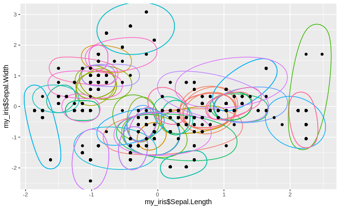
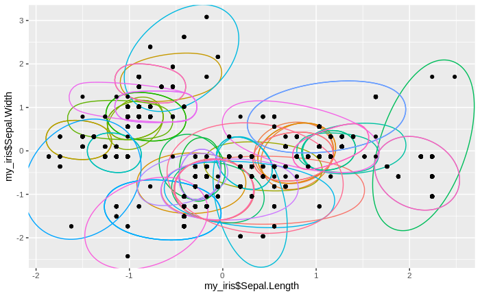
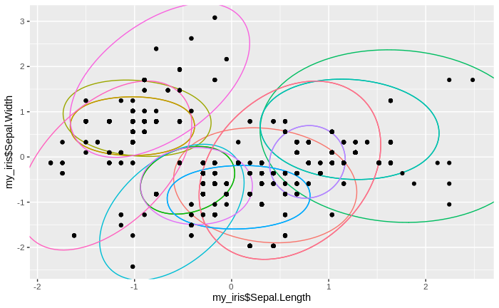
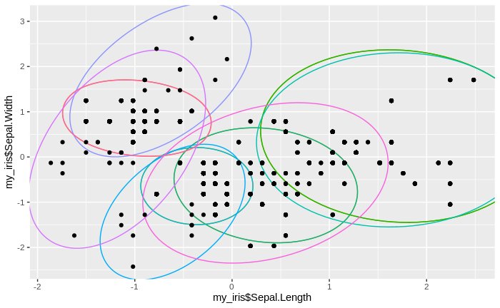
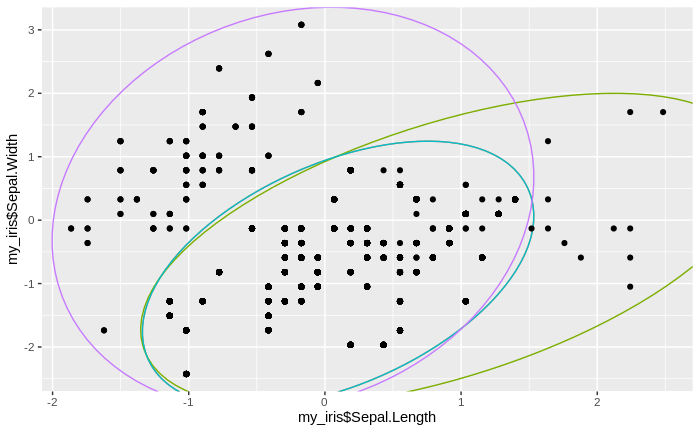
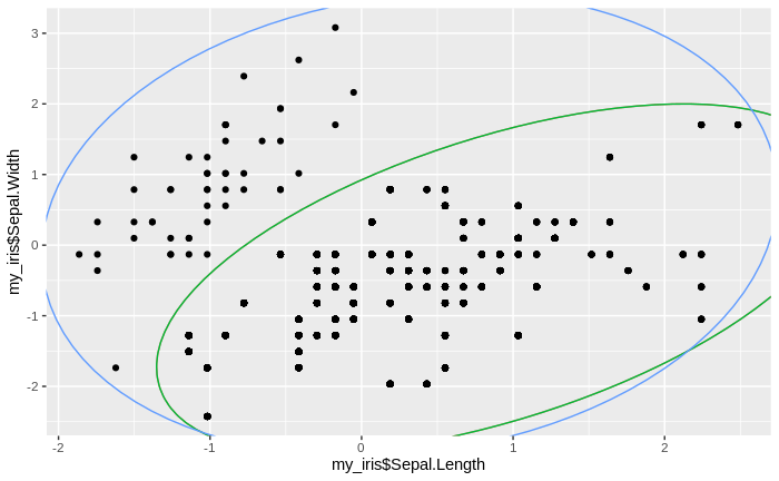
We see that the number of clusters increases, until at some point all data come to lie in just one big cluster. We also see that some clusters tend to merge to larger clusters more quickly than others, and that some separations between clusters are relatively persistent, except for the very final clustering steps.
Of course, we do not want to obtain just one big cluster containing all data. As with the traditional clustering algorithms, the question arises of what is the right number of clusters. While there cannot be an ultimate answer to this question (as it also depends on the context in which the cluster analysis is performed), we can approximate it by applying a technique called "elbow method": remember that in each iteration of the clusteringalgorithm, we recorded the number of clusters, as well as the median sum of differences between cluster means and the data assigned to them. We now plot these median sums against the number of clusters:
plot(n_clusts, mn_diff, 'l');points(n_clusts, mn_diff)
ggplot()+geom_point(aes(iris$Sepal.Length, iris$Sepal.Width, shape = iris$Species))
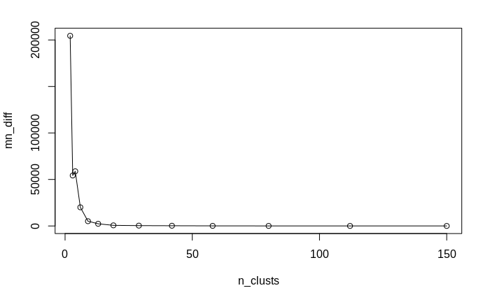
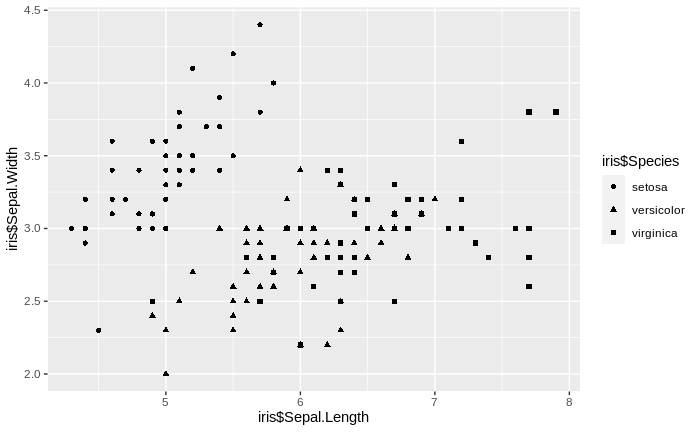
We notice that the relationship is not at all linear; instead, the median sum of differences decreases first very steeply, then much more gradually. The point transition from the steep to the gradual decrease, the "elbow" of the empirical curve, is our approximate "right" number of clusters. This is so since it represents the best trade-off between minimizing the difference between cluster means and the data assigned to them (i.e. maximizing the explained variance) and maximizing the relevance of the clusters (increasing the number of clusters will decrease the non-explained variance, but will lead to many non-relevant clusters, in a similar way as an over-fitted regression model explains the observed data well, but fails to convey information about general relationships). In our case, we find the "elbow" at 13 to 19 clusters. Comparing this clustering scheme to the true classes in the data - the three species - we find that there are actually too many clusters detected by our clustering algorithm. However, the major clusters do show the separation of the three species relatively well, and the overlap region between several major clusters corresponds relatively well to the region in the data where the too species I. versicolor and I. virginica over-lap with respect to the variables sepal length and sepal width.
Hierarchical clustering can thus tell us a bit more about the data than traditional clustering methods like K-means can - the method conveys information about uncertainty in the data, i.e. about regions in the data space where cluster assignments become unclear, or "fuzzy". Ultimately, this can tell us that we should consider measuring more variables than the four employed in order to achieve a clearer clustering of the data.