Clustering with the Expectation-Maximization Algorithm
Expectation-Maximization (EM) is a common clustering algorithm based on probability-density calculations. It is a common alernative to the K-means clustering algorithm
A requirement for the application of EM is that the number of expected clusters is known a priori; furthermore, initial guesses for the mean or center of each cluster have to be provided that are not too far removed from the true cluster means, and that are also not so similar as that the algorithm would not be able to converge on all true cluster means.
Data provided to the algorithm should be normalized (by subtracting the mean and dividing the result by the standard deviation) along each axis (“axis” refers to dimension or variable). This is necessary to avoid convergence issues due to vastly different scales for the different variables. Variables that are likely not to follow a normal distribution should be transformed (e.g. logarithmized), so that the multivariate distribution is Gaussian. The latter should be done before normalization.
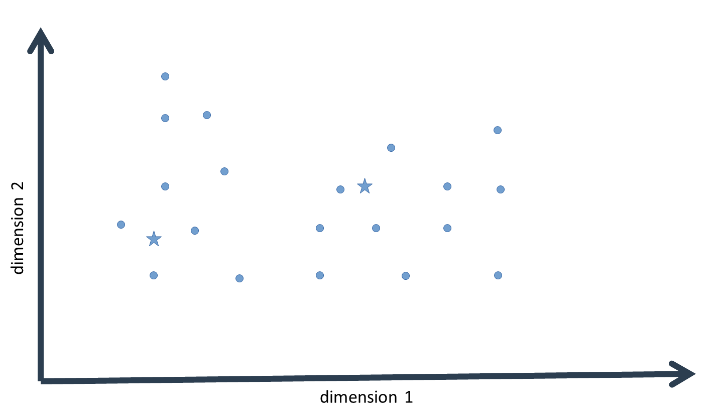
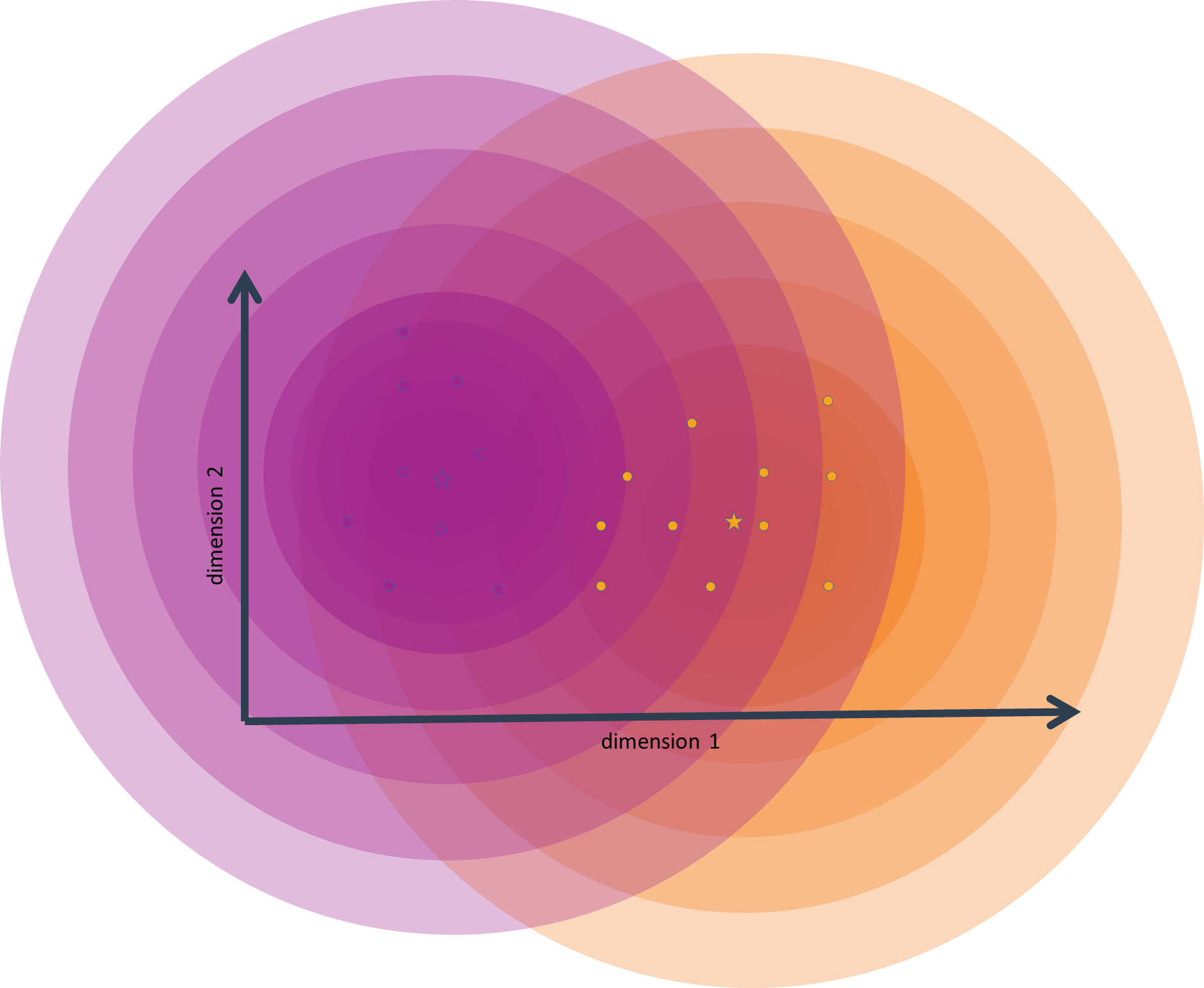
As noted above, the algorithm is initialized by providing initial semi-random guesses for the center or mean of each cluster. This value is a vector with as many dimensions as there are variables in the data, i.e. it is a multivariate mean. For each such mean, we now calculate the probability density of each data-point (vectors with the same dimensionality as the cluster means) on the probability-density function defined by that mean. To do this, it is not sufficient to simply provide the cluster mean. A multivariate distribution – just as a univariate distribution – is always defined by its mean and its standard deviation.
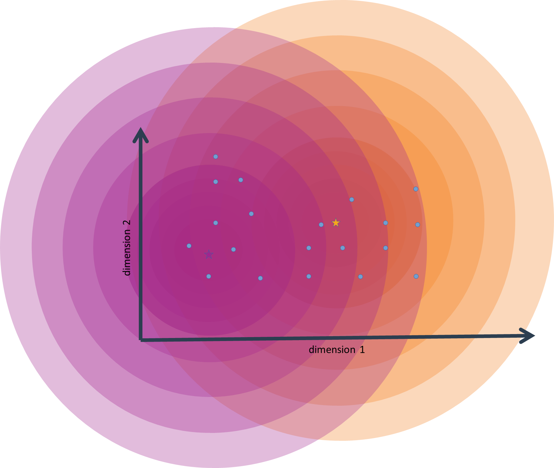
For a multivariate distribution, the standard deviation is called a covariance matrix, or, more inuitively, a variance-covariance matrix. This object is a matrix with as many rows and columns as there are dimensions (variables) in the data. The diagonal values of this matrix (where row and column index are identical) are the standard deviation of each variable. The matrix cells aside from the diagonal are filled with standard deviations from the interaction of a pair of variables. Using the variance-covariance matrix allows us to work with (multi-variate) distributions that are not exactly symmetric.
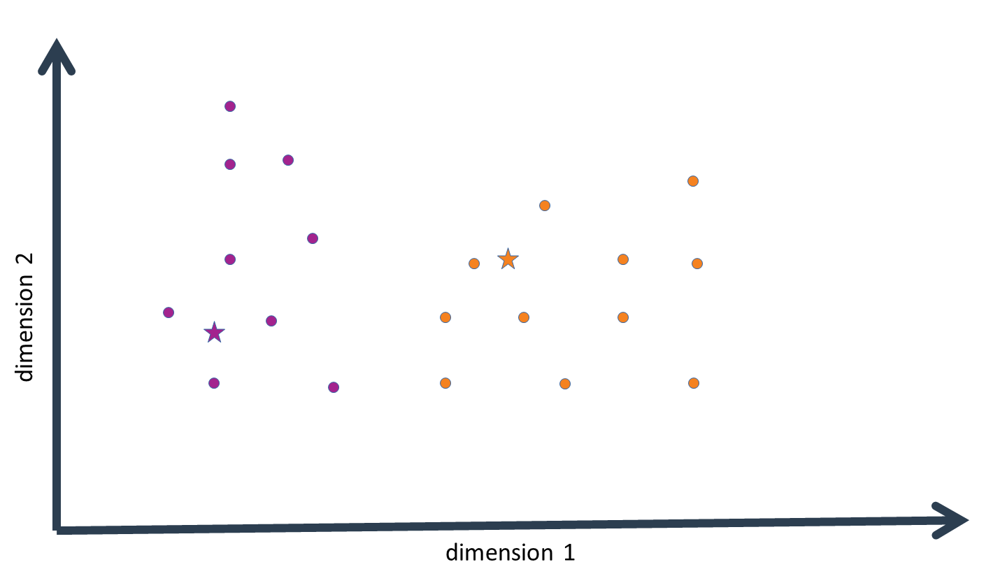
Once multivariate probability densities have been calculated for each "cluster distribution", each data-point is assigned to that cluster for the distribution of which it has the highest probability density value. This results in a first approximation of the clustering structure inherent to our data. We then calculate the mean of the data-points assigned to every cluster. These are then the new cluster centers, i.e. the new cluster means. The cluster means are now a step closer to their true value.
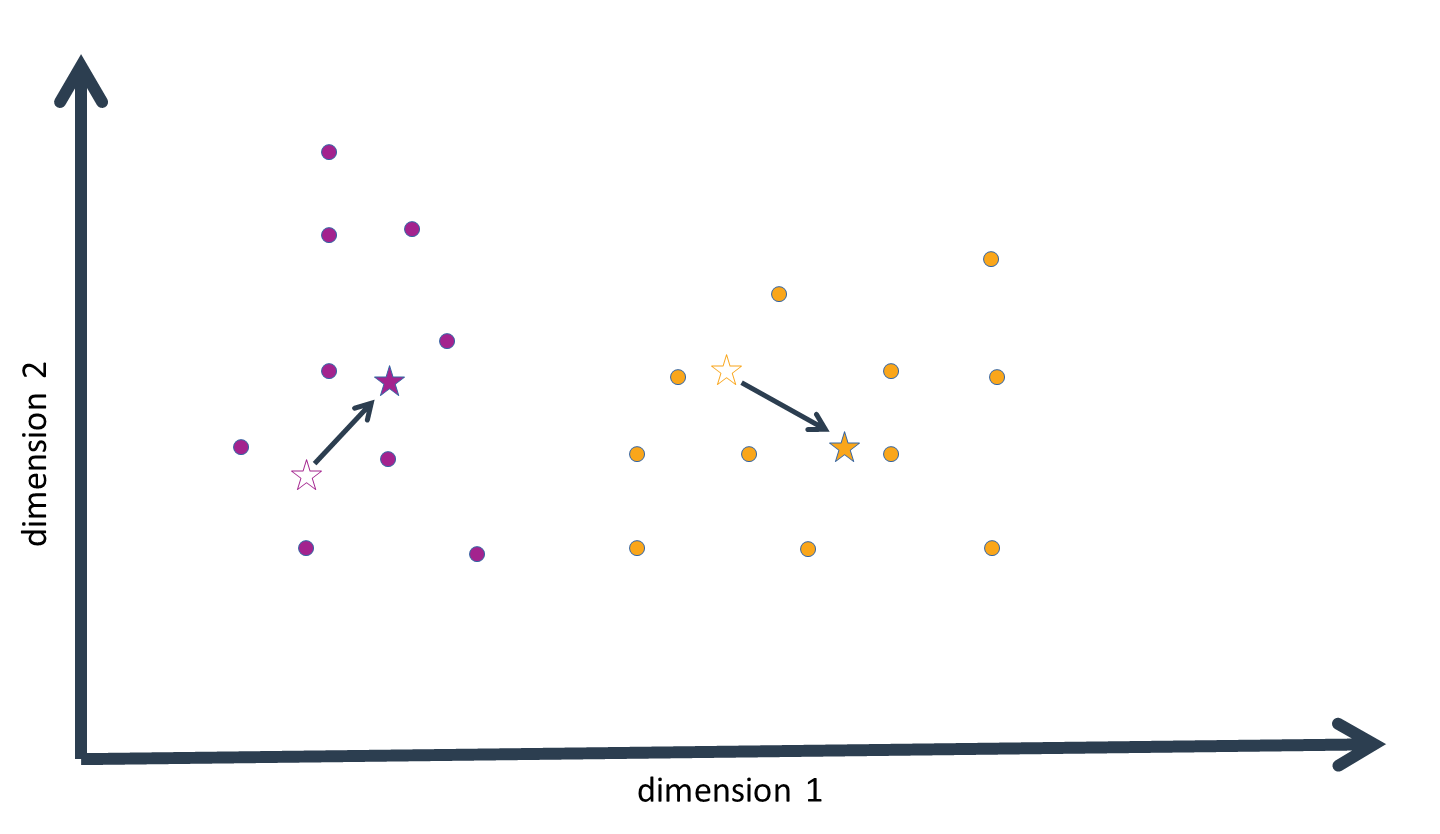
We can now start the second iteration of the EM algorithm; that is, we again compute the probability density of each data-point for the distribution defined by each (new!) cluster mean. It is important to note that the cluster assignments generated in the previous iteration play no role here; they were only intended to generate updated values for the cluster means, and it is entirely possible that the clusters generated in the second and subsequent iterations will deviate from previous clusters.
After a number of iterations, the cluster means will only change by a very small amount between iterations, and clusters will stay largely fixed in composition. This means that the true clusters have now been approximated as well as possible with regard to the constraints imposed on the algorithm (especially with regard to the fixed number of clusters). One says that the algorithm has converged.
We can estimate if the algorithm has converged by computing and plotting the differences between consecutive cluster-mean estimates (summed over all dimensions and cluster means). Once the curve approaches zero (in an asymptotic manner), it is safe to say that the algorithm has converged. The question of how many clusters to expect can be answered to some extent by applying the algorithm to different amount of expected clusters. For each such amount, the algorithm should be run several times with different random starting values. If the resulting clusters are very different among runs, then this is a sign that the number of expected clusters is not realistic (this can be best checked by plotting the clusters along two to three variables of the data). If, on the other hand, the resulting clusters are very similar among runs, it is very likely that the true number of clusters has been found.
Another sign that the number of clusters has been overestimated appears when during a run no data-points are assigned to a specific cluster mean − in this case, the corresponding cluster simply doesn't exist – and so its mean doesn’t exist, either. Another case for this happening can be a strong miss-estimation of the initial-guess value for that cluster mean.
The EM algorithm is closely related to the K-means clustering algorithm, where Euclidean distance is used instead of probability densities to calculate cluster assignments. It is not always easy to tell which of the two algorithms will work better; in the example below, the EM algorithm is applied to the iris dataset, which we know is made up of measurements of three species. In this case, the EM algorithm has a hard time finding the true clusters (especially when there is an unfortunate set of initial random cluster means); here, the K-means algorithm generally works better.
The EM algorithm may be implemented in Python as follows: