Fitting numerical models with Template Model Builder
Fitting the parameters of a complex numerical model can be a daunting task. The Template Model Builder (TMB) package for R is designed for optimizing the parameters in an efficient way. Here, we will look at its impementation on an easy artificial example.
In some applications, model parameters are part of a complex arrangement of equations that describe e.g. a natural system. In such numerical models, a large number of different processes interact to generate predictions of some observable quantity. One example is fish catches, which are typically modelled using a numerical population model, which integrates natural- and fishery-induced mortality processes, as well as the replenishment of the harvested fish stock with juveniles; further extensions can address the growth of individual fish. Parameters for such complex model are often taken from the literature, more specifically from recorded experiments done in the field or in a lab. In some cases, however, parameters might need to be estimated using statistical optimization.
Previous articles have explained optimization procedures in relatively simple settings, where the parameters of one equation were to be fitted in a non-numerical context. These optimization procedures do not require a particularly large amount of computing time (Neural Networks may be an exception, though.). Numerical models, on the other hand, can require a relatively large amount of computing time due to the large number of calculations involved, and the fact that an unpredictable number of iterations of computing model outcome and updating model parameters (via gradient descent) is necessary to achieve convergence in fitting the model (i.e., to achieve a "final state" in the fitting procedure, where deviations between observations and predictions are minimal). The choice of programming language can make a difference in the time required for fitting.
Template Model Builder (TMB) (Kristensen et al., 2016) is an R package written especially for fitting the parameters of complex numerical models. It makes use of the auto-differentiating capability of the computer to generate the partial derivatives of the equations included in the numerical model. These partial derivative equations are necessary to calculate the parameter-specific gradient of the loss generated by the model, i.e. they are essential for updating the parameter values in order to achieve better model predictions. The numerical model itself, or more precisely the calculation of the loss that expresses the (aggregated) deviation between model predictions and observations, is written in a C++ file, which is usually faster than the R programming language at performing the model computations. Output from the C++ operations is fed back to R, where the optimization procedures take place. Note that TMB operations also require the installation of the RTools software, but must be downloaded and installed separately from the web.
Here, we will look at an example application of TMB in the fitting of parameters of a growth model, more specifically the van-Bertalanffy growth model for fish. This model is actually quite simple, and it has an analytical solution, which means that it can be written as a single equation instead of a numerical process of incremental growth over time steps of finite length. The latter is a non-formal description of numerical integration, a procedure applied to calculate integrals (and often estimate prameters along the line) where there exists no analytical solution to a differential equation. The analytical solution of the growth equation would enable parameter estimation using methods described in previous articles (e.g. via the nls fuction in R). However, the numerical expression of the growth process represents an easy, simple example to demonstrate parameter fitting via TMB.
An assumption in many numerical models that describe a natural system is the existence of two sources of unexplained variation (or "error") in the observed data: the first source is the so-called observation error. This is the deviation between observation and reality that results from flawed and non-systematic measurement error, be it due to flawed measurement equipment or difficulties in field sampling. The second source is termed process error. Here, the term "error" is a bit misleading, since the term describes natural variability, i.e. the existence of uncertainty that exists due to the model not capturing every single natural process involved in e.g. growth (and thus being an approximation). Unlike the case with observation error, the process error is part of the natural system one seeks to describe with the model, and the state of the natural system at one time step depends on both its state in the previous time step and on unexplained natural variability. In the example of fish growth, the size of the fish at a given time step depends on both its size at the previous time step and on undescribed additional processes. (this property is one characteristic of so-called state-space models).
The growth equation is characterized by two distinct parameters: i) The length at infinite age of the fish, or Linf. Fish grow in an asymptotic relationship with time, and Linf is the length approximated by the asymptote in later years of age. ii) the slope parameter K, which describes the rate of length increase in the exponential part of the growth curve over time. Linf can be easily visually estimated from the data, while K cannot. In addition, we want to estimate the observation error and the process error. We describe these errors via the standard deviation sigma of these error terms. The two sigmas are treated like two additional parameters, their values are changed to reduce the deviation between observations and model predictions. This procedure requires the application of a different loss functio than the ordinary sum of squared differences (SSQD) discussed in previous articles. This is because SSQD cannot estimate the statistical error, or dispersion, in the data, it can only measure the deviation between predictions and observations, and thus implicitly assumes that the observations represent the reality perfectly.
The "new" loss function is termed negative log-likelihood. The likelihood refers to a probability-density function, which is described by a mean (more on that later) and a standard deviation (often smybolized as sigma). The standard deviation is that of our process error or observation error. In fact, when working with these two error types, we have two "joint" losses, the so-called joint negative log-likelihood. The mean in case of the process-error likelihood function is the model prediction based on the parameters Linf and K to be fitted. In the case of the observation-error likelhood function, the mean is one additional "random" parameter for each data point. These random parameters are basically estimates of fish length without observation error added. Curiously, the process-error equation computes the likelihood of the random parameters based on the model prediction acting as the mean value, while the observation-error equation computes the likelihood of the observed fish length based on the random parameters acting as the function's mean. This linkage of the two equations ensures that both the model"s parameters Linf and K are learnt and that process- and observation errors are estimated properly. The learning of the random parameters is thus more of a side effect, at least in the present case.
The calculated likelihood is logarithmized, which brings it on a scale where it can more easily be optimized (for example, the range of possible values is no longer bounded by zero and one, which is beneficial for optimization algorithms). The negative log-likelihood (i.e. the application of the negative sign function on the log-likelihood) is used since we want to maximize the likelihood (a higher likelihood on the probability-density function implies a closer distance of observation to prediction), but optimization algorithms usually search for the minimum, not the maximum of a function. The joint negative log-likelihood is simply an additive aggregation of the process- and observation-error negative log-likelihoods. In fact, the two likelihoods are calculated for every single data point (requiring one random parameter per data point), and they are then all added up to yield the final loss value passed to the optimization algorithm. In the case of the growth model, the entire growth history must thus be simulated for each iteration of optimization.
In TMB, model fitting requires the writing of two code scripts: The first is a C++ script, which contains the model equations and the calculation of the joint negative log-likelihood. This script must be written very precisely, as it must return one scalar value to the optimizer in R. The second is an R script, which loads the data and initial parameter estimates, and contains the optimization procedures, including the calls to the C++ script. Technically, the processes in R must not necessarily be written as a formal script or program; it is sufficient to start an R session in an IDE like RStudio if one is not working on appication-based programming. We will now look at both scripts, using the example of the fish growth function. Lacking an actual data set of fish length values, and in order to test TMB, we will work with an artificially constructed data set, including controlled addition of process- and observation error.
First, we set values of the parameters of the von-Bertalanffy growth equation: Linf is set to 54.4, K is set to 0.1, the standard deviation defining the process error (here termed sg_p) is set to 0.012, and the standard deviation defining the observation error (here termed sg_o) is set to 0.015. The objective of the model fitting will be to estimate these values "from scratch", i.e. without explicitly passing them to the optimization algorithm. We also set up an empty vector, l_num_int, which we will fill with length values by iteratively applying the first derivative of the growth equation, i.e. by numerical integration. The initial length value needs to be fixed, we set this to 1 (which could be e.g. 1 cm).
set.seed(2)

l_inf = 54.4
K = 0.1
sg_p = 0.012
sg_o = 0.015

l_num_int = vector(length = 100)
l_num_int[1] = 1
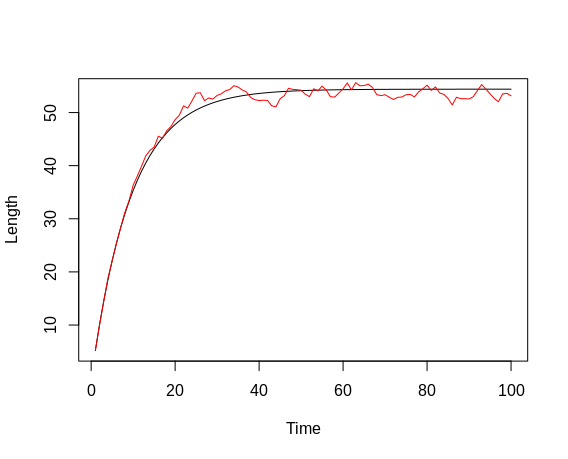
We now iteratively apply the first derivative of the von-Bertalanffy growth equation to generate a time series of length values. The derivative equation has the following form: dL/dt = K * (Linf - Lt), where Lt is the length at time step t. In the first iteration, we start from the initial length of 1 (cm) (at time step 1) defined above. The calculation of length at time step 2 follows a three-step procedure: First, we calculate dL, for which we need to re-arrange the derivative equation to dL = K * (Linf - Lt) * dt. Since we are working with a fixed time step of e.g. 1 week, dt is set to 1. Second, we add the calculated dL to the fish length at the previous time step to generate the "pure" length at the current time step (the fish has grown by the increment dL). Third, we add the process error. As discussed, this term is not an error per se but rather reflects unknown or neglected processes influencing growth. In this example, we assume that the error affects the logarithm of length, hence we sample from a normal distribution where the logarithm of the current length is the mean and sg_p is the standard deviation, and we then exponentiate this value. Biologically, this means that the error is larger at higher lengths, and increases exponentially rather than linearly with length. The process is repeated for a further 198 steps. Plotting the so-generated time series, we see an asymptotic increase in length, with values scattering around the imaginary perfect length-time curve. This scattering is the result of applying the process error.
for(i in 2:100){
  delta_l = K * (l_inf - l_num_int[i-1])
  l_num_int[i] = l_num_int[i-1] + delta_l
  l_num_int[i] = exp(rnorm(1, log(l_num_int[i]), sd = sg_p))
}

plot(l_num_int, type = 'l', col = 'red', xlab = 'Time', ylab = 'Length')
(The method of sampling length from a distribution, rather than adding a value sampled from a distribution, leads to lengths differing in both directions from the length at the previous time step. Whether there truly is a bi-directional process error in fish growth, which would imply temporary shrinking of the fish, is, of course, debatable. Here, this assumption is made in order to provide an easy example of applying and estimating process error.)
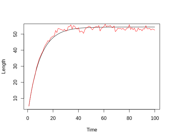
We now take the length time-series and add observation error to each data point. As with the observation error, we sample from a distribution defined by the logarithm of a given length value and the observation-error variance defined above (which means that the error again increases non-linearly with increasing length), and exponentiate that value. Note that this time, the error does not affect subsequent length values, as we do not perform numerical integration here. After all, we only simulate measurement errors here, not unknown effects in fish growth. Once we plot the finalized length values and compare them to those only containing process error, we notice that the scattering of the data now looks slightly different; in addition to the slightly more trend-like deviations, we now observe scattering around these "trends", as the data follow more of a zig-zag line than before.
for(i in 1:length(l_num_int)){
  l_num_int[i] <- exp(rnorm(1, log(l_num_int[i]), sg_o))
}

plot(l_num_int, type = 'l', col = 'red', xlab = 'Time', ylab = 'Length')
We now have everything set up to turn our attention to the C++ script. Writing a C++ script for TMB requires some knowledge about that programming language; nevertheless, given that C++ scripts for TMB tend to follow similar patterns, that requirement has limitations. Of particular importance are some basic rules: First, unlike R, but like Python, C++ starts indexing from 0, not from 1. This becomes important when writing a loop. Second, each line in a C++ script must end with a semikolon (";") in order for the script to work as a self-contained mini-program. Third, subsetting operations use round brackets ("()") instead of angular brackets ("[]"); this is different from both R and Python. The usage of C++ scripts with TMB does not allow experimentation - you have to know what you are writing in the script, and the script either runs or it does not; the error messages returned by TMB after a failed compilation of the C++ script are not informative with regard to the source of the error. As RStudio is (currently) not designed to highlight coding errors in C++ scripts, the best recommendation is to carefully check the script line by line if compilation fails.
  #include <TMB.hpp>
  template<class Type>
  Type objective_function<Type>::operator() ()
  {
    DATA_VECTOR(l_obs);
    PARAMETER(log_sg_p);
    PARAMETER(log_sg_o);
    PARAMETER(log_l_inf);
    PARAMETER(log_K);
    PARAMETER_VECTOR(log_l);

    Type jnll = 0;
    Type pred;
    Type l_inf = exp(log_l_inf);
    Type K = exp(log_K);
    Type sg_p = exp(log_sg_p);
    Type sg_o = exp(log_sg_o);
    vector l = exp(log_l);

    for(int i=1; i<l.size(); ++i){
      pred = log(l(i-1) + K * (l_inf - l(i-1)));
      jnll += -dnorm(log(l(i)), pred, sg_p, true);
    }
    for(int i=0; i<l_obs.size(); ++i){
      jnll += -dnorm(log(l_obs(i)), log(l(i)), sg_o, true);
    }
    return jnll;
  }
Let us now go through the C++ script step-by-step: The first two lines are of purely technical nature and do not require further explanation at this point. The third line is the start of the definition of a function that contains the model whose parameters are to be optimized. That function is named "objective_function" in this case. The procedures contained within the function are written in the indented code block, in-between the curved brackets. It is this function that will later be called by the optimization routines in R. The function is fed with input data and initial guess values for the model parameters, and returns the negative log likelihood to the optimizer algorithm in R. This means that all the model calculations are performed within the C++ function, and thus not directly in the R session. Note that all code lines within the function end with a semikolon; a common mistake when adding or changing code in the function is the unintentional omission of the semikolon. The first couple of rows within the C++ function define the function input expected to be obtained from the R call. The type of input is written in capital letters, while the name of the input follows in round brackets. Here, we have one input of type DATA_VECTOR, these are the observed fish lengths (including process- and observation error, the final result of our generation of artificial data in R above). We have four inputs of type PARAMETER, these are the initial guess values of the growth function, Linf and K, as well as the initial guess values for the standard deviations defining the process- and observation errors, sg_p and sg_o. Note that all these parameters appear here in logarithmized form. This is for practical reasons: The optimizer in R is not bounded, thus it can change parameter values to negative, even if it is not biologically sensible to have negative parameters, or if a negative value leads to undefined results (e.g. when calculating the square-root). Optimizing the logarithm of a parameter averts these issues, since an exponentiation must be done within the function context to obtain the actual parameter value. Exponentiation can never return a negative value, hence the use of logarithms. Finally, we have one input of type PARAMETER_VECTOR, which is the initial guess values for the "pure" fish lengths (without observation error), i.e. the random model parameters.
In the next section, a number of transformations is performed on the input parameters. These operations are all preceded by the term Type, which indicates the creation of a session object (this declaration is never necessary in R or Python). These operations are the aforementioned exponentiations of the logarithms of the parameter guess values (or of the optimized derivates when the script is called upon during optimization). As explained, this is done to avoid having negative values, which could yield non-sensible or undefined model outputs. Two further lines initialize the objects pred, which will be the prediction of the growth function at any time step, and jnll, which stands for "joint negative log-likelihood". The latter object will sum up the process- and observation errors over all time steps of the numerical integration (described above); it is initialized to zero so that there is already one value to which the first process-error value can be added (a simplification of programming).
We now get to the part where the actual model predictions are being made and where the negative log-likelihoods are being computed. Since the joint likelihood is composed of two components, we have two loops: The first loop, in a first step, simulates the procedure of numerical integration described above for calculating predictions of fish length over time (indexed with the symbol i) based on previous fish length. Note the utilization of the parameters l_inf and K defined above. Also note that the procedure here uses the random length parameters (l) as the input to length prediction, instead of the preceding prediction. This is done i) to prevent error propagation through the prediction time series and ii) in order to force the fitting of the random parameters. Each predicted value is actually the logarithm of the predicted length. In a second step, the negative log-likelihood for the current prediction is calculated by computing the value of a probability-density function, defined by the prediction (pred) and the process-error standard deviation (sg_p), for the logarithm of the random length parameter. The dnorm function is utilized to this end, and the argument true lets the function return the logarithm of the probability density. This allows a cumulative addition of the probability density (or likelihood); working with the "pure" likelihood would require cumulative multiplication. Note that a sign function is used to make the log-likelihood negative (optimization usually minimizes a loss). Also note the usage of the += operator, which indicates that the negative log-likelihood for time index i is added to the jnll object, and does not overwrite the existing object (this operator is not available in R). Finally, note that the loop starts from the second time index, 1 (remember that C++ starts indexing at zero), since a preceding length value must be given as input in order to calculate any length prediction. When the loop is completed, the sum of log-likelihood over all time steps but the first has thus been calculated
The second loop calculates the observation-error negative log-likelihood. The synthax is very similar to the calculation of the process-error negative log-likelihood, although in this case one value is also computed for the first time step (index i = 0), since the calculation does actually not involve the calculation of new predictions. In this case, the function of a probability-density function, defined by the logarithm of the random length parameter (l) at time index i and the observation-error standard deviation (sg_o) is calculated for the observed length at the same time index (l_obs). Again, the dnorm function returns the logarithm of the probability density, and a sign function makes it negative. The observation-error negative log-likelihoods for all time steps are all added to the existing jnll object (which at the commencement of the second loop already contains the process-error negative log-likelihood summed over all but the first time step) in order to yield the joint negative log-likelihood. Once the second loop has finished running, the scalar joint negative log-likelihood is returned as the output of the objective_function output. This is the value "submitted" to the optimizer in R, and is thus the basis on which all parameters are adjusted. The first loop can roughly be thought of as existing for the optimization of the the parameters l_inf and K, while the second addresses the random length parameters, though in truth both processes are coupled. According to the documentation of the TMB package, optimization of the random parameters differs from optimization of the "standard" parameters in such a way that the former are optimized separately for each time index i. This is referred to as "integrating out" the random effect. The background to this is that the random parameters are not particularly interesting but are useful to smooth out natural variability in order to more effectively estimate the parameters of interest, namely Linf and K. The parameter sg_p, the process-error standard deviation, serves as some constraint to the inner optimization, since the natural randomness is assumed to follow a probability distribution.
Let us now turn our attention back again at the R session started above. Having finished the C++ file and saved it to disk (using the file ending ".cpp"), we can now proceed to the optimization step. First, we need to load the R package TMB. Then, we compile the C++ script just written using the function compile. According to the official TMB documentation, this creates an object that is shared between R and C++. The operation will fail if there is a technical coding error in the C++ script, though, as noted above, the error message returned does not really give information as to the source of the error. Note that successfull compilation creates two more files in the working directory, with the suffices .o and .so, respectively. Any changes to the C++ script require a re-compilation, which, in my experience, is only successfull when the two automatically-created files are deleted beforehand. A re-start of the R session beforehand (Ctrl + F10) is a useful additional procedure to make sure that TMB starts from a blank slate. Next, we load the shared object using the function "dyn.load". We then create one named list each for the observed data (in this case the artificial measured fish lengths containing process- and observation error) and the parameters (both the target- and random parameters). We set the initial value of each parameter to zero. While optimization in R often requires the provision of sensible initial guess values, in my experience this is not necessary for the present case. Finally, we use the function MakeADFun to create the R objective function to be minimized from the shared R/C++ object created above (using the DLL argument), the data and the parameters. We also need to specify which of the parameters are random (using the random argument). Now, after writing the C++ script, creating the shared R/C++ object and creating the R objective function, everything is ready to start optimization.
library(TMB)
compile("bertalanffy.cpp")
dyn.load(dynlib("bertalanffy"))

data = list(l_obs = l_num_int)
parameters = list(log_sg_p = 0, log_sg_o = 0, log_l_inf = 0, log_K = 0, log_l = rep(0, length(l_num_int)))

obj = MakeADFun(data, parameters, random = "log_l", DLL="bertalanffy")
We now start the optimization using a common optimimzation function, in this case nlminb. This optimization function can be applied to any function that returns a scalar loss value; it is not bound exclusively to TMB. There are a number of different optimizers available in R, which all are essentially different algorithms for performing gradient-descent-based optimization more effectively. In the present case, we need to provide the components par, fn and gr from the objective function ("obj") created above to the optimizer function. Once executed, the optimizer function will iteratively update the parameters in order to decrease the joint negative log-likelihood. As mentioned above, the random parameters are optimized in an "inner" optimization procedure for each time step separately. Once optimization has finished, i.e. once the minimum of the loss function has been approximated, we call the sdreport function, which returns the optimized parameter values and calculates their standard deviations. We can check the report given by nlminb for successful convergence to the minimum of the loss function; in that case, the component convergence of the report given should have the index "0". Optimization can fail when the model function writen in the C++ script is mis-specified, e.g. when NA values or infinite values are calculated and returned as the joint negative log-likelihood (caused e.g. by division by zero). In the present case, efforts were made to avoid the calculation of such values e.g. through the optimization of the logarithms of parameters rather than of the parameters themselves.
fit = nlminb(obj$par, obj$fn, obj$gr)

sdr = sdreport(obj)
We can finally compare the estimated parameter values with the true ones. To this end, we need to exponentiate the vector of parameters (par.fixed) included in the output of the sdreport function. This is because, as mentioned above, the logarithms of the parameters and not the parameters themselves were optimized. We find that the parameters have been estimated quite well, but not perfectly. Providing a longer time series of artificial data might have yielded even better results.
print(cbind(c("sg_p", "sg_o", "l_inf", "K"), c(sg_p, sg_o, l_inf, K), as.vector(exp(sdr$par.fixed))))
Reference: Kristensen, K., Nielsen, A., Berg, C. W., Skaug, H. & Bell, B. M. (2016). TMB: Automatic Differentiation and Laplace Approximation. Journal of Statistical Software, 70, 1-21. doi:10.18637/jss.v070.i05