Support-vector machine for data classification
The support-vector machine is a common algorithm for the classification of data. Here, we take a closer look at the properties of a linear binary support-vector machine.
Classification, like regression, is a major domain in the data sciences. Various algorithms have been developed for predicting the class a data point belongs to, including decision trees and neural networks. One of the most classic methods, though, is the support vector machine (commonly abbreviated as "SVM"). Different from the threshold-based approach of the decision trees, SVMs treat the class prediction as the output of an equation that is, in its simplest form, almost identical to that of a linear regression model, with one parameter associated with each of a selection of variables contained in the data, plus an optional intercept parameter. In the case of binary regression, the SVM's parameters are fitted to predict a "1" for one class and a "-1" for the other. These classes, though, are not treated as discrete factors, but rather as numerics, and of course, the SVM will also predict values in-between 1 and -1 and beyond that range. A sign function is used to derive the predicted class from the numeric output, with positive values indicating prediction of the first class and negative values prediction of the other class.
There is a distinct difference between SVMs and "normal" regression models, though: In SVMs, the goal is to find the optimum hyperplane that separates the data of the different classes. A hyperplane is a separator in the multi-dimensional space containing the data to be classified; in the case of three-dimensional data (data with three numerical variables), it is a plane; in the case of two-dimensional data, it is a line. The hyperplane is defined by the parameters of the SVM equation. A regular fitting procedure would position the hyperplane such as to generate as few mis-classifications as possible on the data available for fitting (often called training data). The resulting hyperplane might, however, generalize poorly and thus make relatively many mis-classifications in applied use. Or it might result in unequal amounts of mis-classifications for the different classes, for example in cases where the hyperplane lies closer to the boundary of one class than to that of another. The fitting procedure on SVMs attempts to make the distance of the hyperplane to all class boundaries as large as possible; this can be interpreted as attempting to increase the width of a "corridor" between the classes, in the center of which resides the hyperplane. During fitting, predictions that fall within this corridor, i.e. predicted values lower than 1 but larger than -1, are treated as uncertain, and the goal is to reduce their number by adjusting the positioning of the hyperplane and its corridor, thereby likely improving generalizability of the SVM.
The parameters that define the hyperplane are thus optimized based on a joint loss function: One part of the joint loss is the sum of mis-classifications, this is simply the sum of the squared differences between predictions made with the SVM equation and the true class indices (1 or -1). Predictions that are larger than 1 or lower than -1 would increase the loss, even though the class prediction is correct when applying the sign function, and are therefore excluded from the summation. Included in the summation are thus wrong class predictions and class predictions of the correct sign that have a modulus of less than 1 and would thus come to lie in the hyperplane's corridor (indicating a likely poor positioning of the hyperplane). The second part of the loss is the width of the corridor around the hyperplane, which we want to increase in order to increase the SVM's generalizing capability. The distance of the hyperplane to the corridor margins is inverse to the magnitude of the SVM parameters [1], and thus the square-root of the sum of squared parameters represents the second part of the joint loss (by decreasing parameter magnitude, the corridor width is then increased).
Let us now look at a custom implementation of the SVM for a binary classification problem on a subset of the iris data set. The iris data set contains four variables and 150 data points, evenly split between three species of the flower genus Iris. For simplicity, we will work with a binary classification task and thus reduce the original data set to two species, setosa and virginica. We then create a class vector, where all indices that correspond to setosa in the data set are assigned a "1", and all those corresponding to virginica a "-1". Also, we make a copy of the flower data set, where we eliminate the Species column, such that we obtain a data set of purely numerical variables. Finally, as is common in many classification- and regression tasks, we standardize the numerical variables in order to give them equal weights (independent of their original scalings). That is, we subtract the mean of a given variable from the value of that variable of each individual data point, and then divide the differences by the standard deviation of that variable.
library('ggplot2')
library('optimr')

iris$Species = as.character(iris$Species)

subs = iris[iris$Species == 'setosa' | iris$Species == 'virginica',]

specs = subs$Species
specs[specs == 'setosa'] = 1
specs[specs == 'virginica'] = -1
specs = as.numeric(specs)

subs = subs[,1:4]

sapply(seq(1,ncol(subs)), function(i){eval(parse(text = paste0(
  'subs$', names(subs)[i], ' = (subs$', names(subs)[i], ' - mean(subs$', names(subs)[i], ')) / sd(subs$', names(subs)[i], ');
  assign("subs", subs, .GlobalEnv)'
)))})
Next, we define a loss function whose parameters can be optimized. Since the SVM is fitted with a relatively complex, joint loss, we cannot use the simple lm function for linear regression here. Rather, we have to write the loss function ourselves and perform the optimization separately using one of R's optimization functions. The function requires a vector of parameters that should be optimized as input. As a first step, it calculates the class predictions via these parameters, using the simple additive equation hinted at above: here, the first parameter is multiplied with the standardized "Sepal.Length" variable, and the second parameter is multiplied with the standardized "Sepal.Width" variable. The two products are added, and a third parameter (corresponding to the intercept in regression) is added. This parameter can be helpful in scaling between the predictor- and the response variable (i.e., the numerical class identity). To keep things simple, and to avoid potential over-fitting, we limit ourselves to two predictor variables in the current case. (In real-world cases, it would be best to try out different combinations of all available variables, in order to generate the optimum classification algorithm.) Note that we do not apply the sign function here, since for calculating the loss, we need to treat predictions with values with a modulus larger than 1 differently from the rest.
opt_probl = function(pars){
  preds = pars[1] * subs$Sepal.Length + pars[2] * subs$Sepal.Width + pars[3]
}
We next multiply every prediction with its corresponding true numerical class label, and subtract the product from 1. Afterwards, we set all negative differences to zero. This has the following reasons: If the prediction and the true class label have the same sign, and their product is larger than one (i.e. the prediction is correct and is not in the corridor around the hyperplane), subtracting that product from one will yield a negative value, and that will be increased to zero. Effectively, the prediction does not contribute to the overall loss, since it is correct and far away from the hyperplane. If the signs of the prediction and the class label are not identical, the difference will always be greater than zero, and will contribute to the overall loss, since the prediction is obviously wrong. If the signs are equal, but the prediction is less than 1 and greater than -1, the difference will also be positive, and will contribute to the overall loss. This is because the prediction, though correct, lies in the corridor around the hyperplane, i.e. uncomfortably close to the area of the other class. This indicates that the hyperplane may not be positioned well enough to ensure that unseen data points have a high chance of being classified correctly, even though the majority of the data points used for fitting were. Finally, the losses calculated for the individual data points is summed up. We have now obtained the first component of the joint loss.
opt_probl = function(pars){
  preds = pars[1] * subs$Sepal.Length + pars[2] * subs$Sepal.Width + pars[3]

  loss = 1 - specs * preds
  loss = unlist(lapply(seq(1, length(loss)), function(x){max(c(0, loss[x]))}))
  loss = sum(loss)
}
The second part of the joint loss is calculated as the square-root of the sum of the squared parameter values. Here, we only include the parameters that are multiplied with variables of the data. As noted above, the width of the corridor around the hyperplane if inverse to the magnitude of the parameter values, so by decreasing them, the corridor width is increased. We finally add up the two components of the joint loss, which are then returned as the scalar output of the function. The goal of optimization is now to reduce that value by altering the parameters defining the positioning of the hyperplane.
opt_probl = function(pars){
  preds = pars[1] * subs$Sepal.Length + pars[2] * subs$Sepal.Width + pars[3]

  loss = 1 - specs * preds
  loss = unlist(lapply(seq(1, length(loss)), function(x){max(c(0, loss[x]))}))
  loss = sum(loss)

  loss_2 = sqrt((pars[1])**2 + (pars[2])**2)

  loss = loss + loss_2

  return(loss)
}
We now apply the optimization function on the binary classification problem inherent to the data set prepared above. We assign a start value randomly drawn from a normal distribution to each of the optimizable parameters - the two slopes and the intercept. Then we call the optimr function included in the R package of the same name, and pass a vector of the parameter start values that we just defined, and the name of our loss function. After completion of the optimization (this happens in an instant in this case), we extract the parameters and use them to generate class predictions: To this end, we simply write down the prediction function from the loss function and insert the parameters just extracted (replacing the "placeholders" from the function context). Also, we embed the function within a sign function in order to generate categorical class predictions ("+1" or "-1").
set.seed(9)

w1_start = rnorm(1)
w2_start = rnorm(1)
b_start = rnorm(1)

optimz = optimr(c(w1_start, w2_start, b_start), opt_probl)

pars = optimz$par

dat_preds = sign(pars[1] * subs$Sepal.Length + pars[2] * subs$Sepal.Width + pars[3])
Now, we also want to know where exactly the hyperplane is situated, which will not be directly revealed from the predictions, which cover only a limited part of the variable space. So, in order to better approximate the hyperplane, we create a vector of 100 evenly spaced values for each of the two predictor variables, each covering the range between the minimum and the maximum value of the (standardized) variable. Then we apply the prediction function to each unique pair of values from the two vectors. We use vectorized prediction-making here by iteratively combining the full vector of one variable with one element of the vector of the other variable - the result is a matrix of predictions. For each column in the prediction matrix (with each column representing one consecutive entry in the vector of the first predictor variable), we determine the row index of the minimum prediction that yields class "1". Then we subset the column of the second predictor variable with this index, and thus obtain, for this variable at the specific value of the first predictor variable, the threshold value at which the class prediction switches between the two classes. This scalar value is added to an empty vector of length equal to that of the variable vectors (with the added condition that the index should not equal 1). When the procedure has been completed for every entry in the first predictor variable (i.e. every column of the predictions matrix), we have obtained a good estimate of the position of the hyperplane within the variable space.
x1 = seq(min(subs$Sepal.Length), max(subs$Sepal.Length), length.out = 100)
x2 = seq(min(subs$Sepal.Width), max(subs$Sepal.Width), length.out = 100)

pred_var = cbind(x1, x2)

preds = matrix(nrow = length(x2), ncol = length(x1))

for(i in 1:length(x1)){
  preds[,i] = sign(pars[1] * x1[i] + pars[2] * x2 + pars[3])
}

hyp_p = vector(length=100)

for(i in 1:100){
  hyp_p[i] = ifelse(min(which(preds[,i] == 1)) == 1, NA, x2[min(which(preds[,i] == 1))])
}
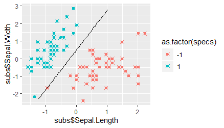
Finally, we plot the observed data and the class predictions, as well as the position of the hyperplane. We utilize the ggplot function to this end, and add two scatter-plot layers with different shapes: a round dot for the observations, and an "x" for the predictions. Further, we add a line-plot layer to draw the hyperplane, where we set the vector for the first variable used in the estimation procedure described above as the x-variable and the vector of threshold values as the y-variable. We find that all data points were classified correctly, and that the hyperplane is quite far away from both classes. However, we also see that one data point belonging to the "-1" class lies almost on top of the hyperplane, and that one belonging to the "1" class is much closer to the hyperplane than the rest. These two data points have, however, a relatively large distance to their class clusters, appearing to be outliers with respect to one predictor variable.
ggplot() +
  geom_point(aes(subs$Sepal.Length, subs$Sepal.Width, color = as.factor(specs))) +
  geom_point(aes(subs$Sepal.Length, subs$Sepal.Width, color = as.factor(dat_preds)),
             shape = 4, size = 2, fill = NA) +
  geom_line(aes(x1, hyp_p))
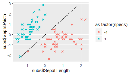
We can now test how the SVM behaves when the second component of the loss function, which optimizes the positioning of the hyperplane with respect to increasing the distance to the classes and thus to increasing generalizability, is not incorporated. We simply need to remove a few lines of code from the loss function, and run the rest of the code as described above.
opt_probl = function(pars){
  preds = pars[1] * subs$Sepal.Length + pars[2] * subs$Sepal.Width + pars[3]

  loss = 1 - specs * preds
  loss = unlist(lapply(seq(1, length(loss)), function(x){max(c(0, loss[x]))}))
  loss = sum(loss)

  return(loss)
}
When we compare the plot showing the predictions and the hyperplane to that of the true SVM we find that, although all data points were again classified correctly, the hyperplane is now much closer to the "-1" class. In fact, the distance of the hyperplane to the class clusters is now much more unequal, so that we can expect more mis-classifications of unseen data points belonging to the "-1" class. This observation thus highlights the advantage of the SVM over simpler classification algorithms that are optimized simply by reducing the number of mis-classifications.
[1] https://math.stackexchange.com/questions/1305925/why-is-the-svm-margin-equal-to-frac2-mathbfw