Building classification- and regression trees from scratch
Classification- and regression trees are a common technique for "mining" complex data sets for information. Here, in order to shine some light on these often blackbox-like algorithms, we have a thorough look at some custom-written trees.
Tree-based machine learning is a popular technique due to the relatively simple interpretability of the concept: A given data point is subjected to a sequence of "questions", and depending on the "answer" (mostly "yes" or "no"), it is sent to the next node in the tree, where the next question is asked. Eventually, the data point ends up on a "leaf" of the tree, where it is separated from some or all other data points, and no further questions are asked. This common image conceals, in my opinion, some of the original ideas behind classification- and regression trees, and reads somewhat different from the otherwise very straightforward-written descriptions of data-mining algorithms: The key idea behind the algorithm is to divide a data set into a hierarchically-ordered set of bins in order to create subsets, based on the observed properties (variables) of the data. These subsets could be dominated by a specific class; then the algorithm would work as a classification mechanism. Or the subsets could represent a specific level (with variability) of a quantitative response variable, then the algorithm would work as a regression mechanism. In applied use, new data points (of which the class or value of the response variable is unknown) would be assigned to a bin based on the values of the observed variables, and the dominating class or mean response value of that bin would be predicted. This also means that tree algorithms cannot predict classes or response values for data points whose properties are outside the range of values covered in the creation of the tree, unlike e.g. linear regression models, which can do this. Due to the property of the tree algorithms to "split" a data set, I prefer the image of a breaking mirror (with the shards as the subsets) instead of a growing tree.
We will now look at an implementation of a classification tree "from scratch". Even though classification trees are not uncommon to find as readily-available functions for R and Python, it can be enlightening to try programming one by one-self. One word of caution, though: There is no guarantee that the procedures shown in the following accurately replicate the implementation in the commonly available packages. What is shown here is more of an own implemnentation of classification-tree theory. We will build a classification tree for the common iris data set, which is included in the basic R environment and consists of 150 measurements of four variables (lengths and widths of flower leaves), assigned to three species of the genus Iris. The task is to build a classifier that can assign a flower to the correct species based on the measurements on a plant's flower. In the present case, we reduce the iris data set to just two species (i.e., observations 51 to 150) for demonstrative purpose. We start by standardizing each variable in the data set, i.e. we subtract the mean of each variable from the single measurements and divide the result by the standard deviation of the respective variable. This operation is meant to avoid unintentional higher weighting of variables with comparatively high moduli.
library('tidyverse')
library('viridis')

iris_std = iris[51:150,]

sapply(seq(1,4), function(x){eval(parse(text = paste0('iris_std[,',x,'] = (iris_std[,',x,'] - mean(iris_std[,',x,'])) / sd(iris_std[,',x,'])'))); assign('iris_std', iris_std, .GlobalEnv)})

iris_std$Species = as.character(iris_std$Species)
Next, we define a function that splits a data set, or a subset thereof, into two new subsets, according to a threshold value in one of the four variables of the iris data set. This function will later on be supplied to an optimizer function, which will change the threshold value such as to increase the purity of the subsets, or to decrease the number of observations that do not belong to the dominating species of the subset. To this end, the function first creates the two subsets ("subs_1" and "subs_2") by logical subsetting of the supplied data set ("subs"), where one of the new subsets receives all observations whose values for the current variable lie below the threshold, and the other subset receives all observations whose values are equal to or larger than the threshold. Note that the threshold is uni-dimensional, since the idea of the three is that the different variables will be looked at in sequence, i.e. in a hierarchical (and often recursive) manner. We next calculate, for each subset, the number of instances where the species (the fifth column in the data) is not equal to that of the majority of observations in a given subset (i.e., the first entry in the list of species sorted by amount of occurrences). These sums are termed "l1" and "l2" in the current example. The total sum ("l1" + "l2") is returned as the function output, and is the loss to be minimized by changing the threshold value. Note that the function is here written for a binary classification problem; multi-class classification problems would require the optimization of multiple threshold values, and the data set would be split into more than two subsets.
split_data = function(spl_est, subs, var_ind){
  subs_1 = subs[subs[,var_ind] > spl_est,]
  subs_2 = subs[subs[,var_ind] <= spl_est,]

  l1 = sum(subs_1[,5] != names(sort(table(subs_1$Species),decreasing=TRUE))[1])
  l2 = sum(subs_2[,5] != names(sort(table(subs_2$Species),decreasing=TRUE))[1])

  return(l1 + l2)
}
Now, we apply the splitting function for the first time on the - at this point still entirely complete - data set. We set the index of the variable (or of the column in the data set) along which we want to split the data, to 1 (this corresponds to the "Sepal.Length" variable). We utilize the optimize function to find the value that splits the data optimally along the current variable, i.e. that yields the purest-possible subsets in terms of the species included in each subset. You may recall that the optimr function was used for optimization purposes in earlier chapters, but since we have a one-dimensional optimization problem at hand for the moment, it is reasonable to use optimize, which was specifically designed for one-dimensional optimization problems. The arguments we pass to optimze are the following: the name of the function to be optimized (split_data), the interval in which the splitting threshold should lie (here we simply set the minimum and maximum value of the current variable as the boundaries of the interval), and two extra arguments that will be passed down to split_data: the name of the data set or subset to be split (this is at the moment the full data set, iris_std), and the index of the variable along which to split (this is the index 1, or curr_ind). The optimum threshold found by the optimization function is contained in the "minimum" slot of its output.
curr_ind = 1

opt = optimize(split_data, interval = c(min(iris_std[curr_ind]), max(iris_std[curr_ind])), subs = iris_std, var_ind = curr_ind)
spl = opt$minimum
We now create a list ("spl_list") that contains two elements: first, all the data whose "Speal.Length" is larger than the optimized threshold, and second all the data whose "Speal.Length" is equal to or smaller than the threshold. The idea on how to proceed from now is to take each element and split it into two sub-units, via optimization, as well. This operation will then be continued quasi ad infinitum, or until each subset only includes one data point and cannot be split anymore. All the while, the variable along which splitting occurs will be varied: in the present example, the four variables will be used in sequence, and once the fourth variable ("Petal.Width") has been used, we will go back to the first. There is, of course, no particularly good reason to start with the first variable in the data, but then again there is no common rule on which variable to start with. Real-world applications of classification trees therefore actually use a combination of trees, where the sequence of variables is randomized in each. This multi-model approach is termed Random Forest. Furthermore, we initialize another empty list ("spl_list_all"), which will be used to record all the subsets created in any of the subsequent splitting operations. It will be used later on to visualize the splits in the data. Accordingly, we assign the list created above as the first element in this "recordings list".
spl_list = list(iris_std[iris_std[,1] > spl,], iris_std[iris_std[,1] <= spl,])

spl_list_all = vector('list')
spl_list_all[1:(length(spl_list))] = spl_list
Next, we write a loop that performs the iterative splitting in a generalized scheme. Hence, we only need to run the loop once to perform all splits in the entire data set. To this end, we first write an inner loop that iterates over every element in the list containing the subsets created in the last splitting operation ("spl_list"). What we want to do for every subset is to perform a splitting operation as described above for the whole data set. We do, however, need to make this procedure conditional i) on the existence of more than one data point in the subset at hand (otherwise, there is no point in trying to split; i.e. a terminal "subset", or "leaf", has been reached) and ii) that the minimum and maximum values of the varible along which to split are not identical. Not fulfilling the latter condition does not necessarily mean that there is only one data point in the subset; nevertheless it is impossible to split the data along that variable if there is no range of values defined for it. If both conditons are fulfilled, then the subset is split along the variable of the subsequent index relative to the prior one (so in the first iteration it is the second column in the data, "Sepal.Width"), using again the optimize function. Note that we now supply the xth element of the list containing the subsets of the first splitting ("x" being the loop index) as the data on which to perform the new split, and the prior variable index ("curr_ind") increased by 1. We create a new empty list ("spl_list_next") and immediately add the two new subsets, i.e. the data lying above or below the threshold computed via the optimization. Note that the new list is only initialized during the first iteration, as it is to be filled with new subsets while looping over the prior subsets. After the loop is completed, the list will, at the present stage, contain four subsets; two from the first original subset and two from the second one.
for(x in 1:length(spl_list)){
    if(x == 1){spl_list_next = vector('list')}

    if((nrow(spl_list[[x]]) > 1) & (min(spl_list[[x]][,curr_ind+1]) != max(spl_list[[x]][,curr_ind+1]))){
      opt = optimize(split_data, interval = c(min(spl_list[[x]][,curr_ind+1]), max(spl_list[[x]][,curr_ind+1])), subs = spl_list[[x]], var_ind = curr_ind+1)

      spl_list_next[[length(spl_list_next)+1]] = spl_list[[x]][spl_list[[x]][,curr_ind+1] > opt$minimum,]
      spl_list_next[[length(spl_list_next)+1]] = spl_list[[x]][spl_list[[x]][,curr_ind+1] <= opt$minimum,]
    }
  }
When the optimization for the final subset of the prior list of subsets has been completed, a number of additional procedures is performed (hence we make them conditional on "x" equaling the length of "spl_list"): First, we increase the variable index by one. During the initial loop, the index was 1, and the optimization on both subsets utlized the index #2, hence in the next round, the splitting of the data will go along the variable with index #3. Since there are only four variables, we need to reset the index to zero once the current index has been increased to four (hence, in the subsequent loop, splitting will again occur along the variable indexed with "1"). This only becomes an issue in the third loop, and then in every fourth loop going forward. Next, we add the new list of subsets ("spl_list_next") to the list that records all the subsets created in every splitting operation, "spl_list_all". (Here, we impose the additional condition that "spl_list_next" must have content in order to avoid an error message; "spl_list_next" can be empty if all previous subsets contained only one data point). Finally, we overwrite the original list containing subsets ("spl_list") with the one containing the collection of new subsets resulting from the loop ("spl_list_next"). This is an important preparation for calling the loop anew: By now, we have created two subsets for each of the two initial subsets, and we have saved all four new subsets to the list "spl_list_next". The initial subsets are no longer required, we are now only interested in the four new subsets. Since the subsets collected from all prior subsets are now collected in one list, we simply need to call the loop again, and we do not need to make any changes to the operations performed in the initial loop.
for(x in 1:length(spl_list)){
    if(x == 1){spl_list_next = vector('list')}

    if((nrow(spl_list[[x]]) > 1) & (min(spl_list[[x]][,curr_ind+1]) != max(spl_list[[x]][,curr_ind+1]))){
      opt = optimize(split_data, interval = c(min(spl_list[[x]][,curr_ind+1]), max(spl_list[[x]][,curr_ind+1])), subs = spl_list[[x]], var_ind = curr_ind+1)

      spl_list_next[[length(spl_list_next)+1]] = spl_list[[x]][spl_list[[x]][,curr_ind+1] > opt$minimum,]
      spl_list_next[[length(spl_list_next)+1]] = spl_list[[x]][spl_list[[x]][,curr_ind+1] <= opt$minimum,]
    }

    if(x == length(spl_list)){
      curr_ind = curr_ind+1
    }
    if(curr_ind > 3){curr_ind = 0}

    if(x == length(spl_list) & length(spl_list_next) > 0){
      spl_list_all[(length(spl_list_all)+1):(length(spl_list_all)+length(spl_list_next))] = spl_list_next
    }

    if(x == length(spl_list)){
      spl_list = spl_list_next
    }
  }
Since we do not know before at which point there will be no more subsets to split, we embed the loop in a while() condition: As long as the "spl_list" contains at least one element, the loop will be executed. In the end, we receive a list ("spl_list_all") that contains all subsets ever created during the multiple executions of the loop. This enables us to visualize all subsets at once, and thus also the splitting thresholds applied.
while(length(spl_list) > 0){
  for(x in 1:length(spl_list)){
    if(x == 1){spl_list_next = vector('list')}

    if((nrow(spl_list[[x]]) > 1) & (min(spl_list[[x]][,curr_ind+1]) != max(spl_list[[x]][,curr_ind+1]))){
      opt = optimize(split_data, interval = c(min(spl_list[[x]][,curr_ind+1]), max(spl_list[[x]][,curr_ind+1])), subs = spl_list[[x]], var_ind = curr_ind+1)

      spl_list_next[[length(spl_list_next)+1]] = spl_list[[x]][spl_list[[x]][,curr_ind+1] > opt$minimum,]
      spl_list_next[[length(spl_list_next)+1]] = spl_list[[x]][spl_list[[x]][,curr_ind+1] <= opt$minimum,]
    }

    if(x == length(spl_list)){
      curr_ind = curr_ind+1
    }
    if(curr_ind > 3){curr_ind = 0}

    if(x == length(spl_list) & length(spl_list_next) > 0){
      spl_list_all[(length(spl_list_all)+1):(length(spl_list_all)+length(spl_list_next))] = spl_list_next
    }

    if(x == length(spl_list)){
      spl_list = spl_list_next
    }
  }
}
We can now plot the whole data set and all the subsets simultaneously, which also highlights the threshold values along which the splits were performed. To this end, we will utilize the list containing all subsets created during the multiple runs of the splitting loop ("spl_list_all"). Each element of that list is one subset of the original data set, and hence shares its structure: four columns of standardized variables, and a variable number of rows (the number depends on the number of data points included in any given subset). We want to plot the subsets with ggplot. We create a long sequence of ggplot layers in form of an expression that will later on be evaluated, i.e. executed. Each layer is a geom_rect layer, which means that it draws a rectangle, whose limits on the x- and y-axes we specify. We will first plot the data in terms of the first and second variables (the "Sepal" variables), hence we supply the minimum and maximum of the first variable in a given subset as the borders of its rectangle on the x-axis. We supply the minimum and maximum of the second variable as the borders on the y-axis. Finally, we select a color for the rectangle. We pick a color from the viridis color range, whose length is set to equal the number of subsets. This will enable us to differentiate earlier from later splittings of the data. We iterate over all elements of "spl_list_all" (indexed with "x") using the sapply formulation. We connect the single expressions with a "+" using the paste0 function.
xpr = paste0(sapply(seq(1,length(spl_list_all)), function(x){paste0(
  'geom_rect(aes(xmin = min(spl_list_all[[',x,']][,1])-0.1, xmax = max(spl_list_all[[',x,']][,1])+0.1, ymin = min(spl_list_all[[',x,']][,2])-0.1, ymax = max(spl_list_all[[',x,']][,2])+0.1), color = viridis(length(spl_list_all))[',x,'], fill = "transparent")'
)}), collapse = ' + ')
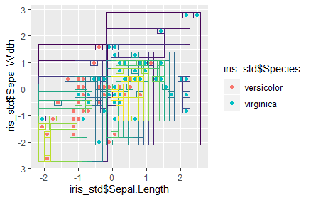
Next, we add the leading ggplot() expression, as well as a scatter-plot layer that will draw the data points of the whole data set, in front of the concatenated rectangle-layer expressions. Finally, we execute the completed expression as a command using the eval and parse functions. The plot created shows us the full data set, with the first variable on the x-axis and the second variable on the y-axis. We also see several rectangles, which indicate the threshold values in the x- and y-variables along which the data were split into subsets. The color of the rectangles indicates whether a given subset was created earlier or later in the process; brighter colors correspond to a later creation. We can observe that almost every data point is now included in its own bin. In applied usage of classification trees, one would limit the number of bins (or "leaves") a priori, in order to main an acceptable degree of generalizing capability of the algorithm (with only one or two data points included in one bin, minor variability to the separation of classes in the full data set could lead to major classification error if the unique or dominating class in a given bin is used for classification of unlabeled data points - hence it is more appropriate to work with larger bins, where variability is "smoothed out" by determining the dominating class for classification tasks).
xpr = paste0('ggplot() +
  geom_point(aes(iris_std$Sepal.Length, iris_std$Sepal.Width, color = iris_std$Species)) + ', xpr)

eval(parse(text = xpr))
We have thus finished our classification tree. Regression trees work quite similarly, though the loss function measures the Euclidan distance of all data points from the mean of the subset, and the optimizer function attempts to reduce that summed distance, in order to find good splitting thresholds in the data.