ExDataScientia

Convolutional Neural Networks

Convolutional Neural Networks (CNNs) are today's gold standard for image classification and Machine Vision in general. By simulating the procedures in which visual input is processed in the human brain, CNNs often outperfrom traditional Deep Neural Networks.

So what is it that makes CNNs so special? To answer that, it is necessary to have a look at the inner workings of these networks, and how they differ from traditional Neural Networks (NN): In traditional NNs, any input is in the form of a vector, i.e. a one-dimensional data struture. This dimensionality is maintained through all data representations that are generated in subsequent layers, and in the output (except the case where the output is a scalar value, as in regression or binary classification). By their very nature, images are not one-dimensional in strcture, but two-dimensional (in gray-scale images) or three-dimensional (in color images). Therefore, when images are supplied to a classic NN, and their structure is reduced to one-dimensional, information is lost. That - spatial - information is often critical for successful image classification, however. This is easily understandable when trying to make sense of an image that exists as a long line of pixels as a human: You would need a lot of training trying to interpret such input!

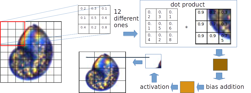
CNNs solve the drawback of classic NNs by mainataining the original dimensionality of the structure of the input. Indeed, no transformation except a scaling to square format is performed (and even the squaring can be circumvented, though only with a lot of effort). CNN parameters, also known as weights, which project the input into a lower-dimensional representation, are arranged in spatial fields, as well: The weights are arranged in a stack of relatively small matrices, which often only have two to four rows and columns. Each matrix "slides" over the image, such that an area of the same extent as that of the matrix is "covered" at a time. Each input pixel value is multiplied with the weight of the weight matrix that is "covered" by at a given time. The input-weight products so generated are then summed up (this is the dot product of the weight matrix with the area of the input it currently overlaps with), and a bias (offset) is added. This sum represents the first element in the first hidden representation of the input. If we started sliding the weight matrix at the top left corner of the input image, then this element is also in the top left corner of the first matrix of the hidden representation.

The weight matrix then moves by one or more pixels (that number is determined by the CNN designer, and is referred to as the stride length), and the same operation - the calculation of the dot product from weights and pixel values - is repeated. By moving the weight matrix over the entire extent of the input image (which is essentially one big matrix in the case of gray-scale images, or a stack of three matrices in the case of color images) step by step, the first part of the first hidden representation is generated. Structure-wise, this partial hidden represenation is a matrix, just like the input. Spatial information of the input is thus retained in the hidden representation. Usually, more than one weight matrix is "slid" over the input; instead, the number can be quite high. Baseline CNNs often feature hundreds of weight matrices even in the first hidden layer. For each weight matrix, there exists a corresponding matrix in the hidden representation generated by the layer employing these matrices. Effectively, the hidden reprsentation is thus a stack of matrices, or a three-dimensional array.

Each of these weight matrices "scans" the image for a distinct feature, like an edge, a curve, an angle and so on. Since we are dealing with a Neural Network, we don"t need to pre-specify what these features are; instead, they are derived from the data themselves in the training process: After processing the input image through the CNN, the output classification is compared with the true classification by applying a loss function on the two. The CNN weights are then updated by gradient descent in response to the loss incurred. Through the loss-driven adaptation of the weights, the CNN learns what features to scan for in the input image (by the way, this also means that what is learned to be recognized depends a lot on the task at hand, and ultimately on the way we, the model designers, have classified the images). The number of weight matrices employed thus depends on the complexity of the images we want to train the CNN on, and on the number of features we expect to be necessary for a good classification rate. A hidden layer that employs weight matrices in called a convolutional layer; the process of multiplying weights of a matrix with the weights of the over-lapping pixels is termed the convolution.

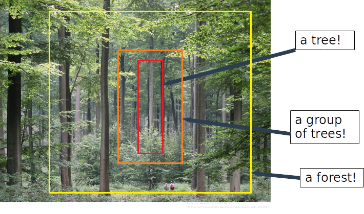
Often times, images are so complex that they contain that we could call hierarchical features: The image of an eye could be described to consist of circles and curves; a human face then consists of eyes, nose and mouth; a human consists of face (head), body, arms and legs (in a very reduced description). The CNN should ideally be able to learn all these hierarchical features to be able to classify complex images. For this reason, a CNN usually contains not only one, but several hidden layers. Each hidden layer can be considered as one "level" in the hierarchy of features. Thus, a hidden layer close to the input layer may scan for edges, curves and so on, while a layer relatively close to the output may scan for faces, hands and feet. In each hidden layer, each weight matrix represents one such feature. The connective nature of NNs means that these features are learnt simultaneously; the weight updates are performed in every hidden layer in response to the loss given by comparing predicted classification with true classification. In practice, however, it has been shown that the isolated training of select layers can be advantageous. Also, the recognition of features in an explorative manner (via auto-encoding), separate from the constraint of classification, has been shown to improve the training of CNNs.

CNNs do not only contain of convolutional layers. In fact, even in basic CNNs the convolutional layers are arranged in blocks of two to three; these layers learn features of similar "extent" in the image (for example, a ear and an eye are of similar extent given their similar size with respect to the position of the camera which took the image). These blocks are separated by the so-called pooling layers. These layers are weight-less, they simply sum the values of a certain area of a hidden representation. Compared with convolutional layers, the dimensionality reduction in pooling layers is quite drastic; oftentimes, the "edge lengths" of the matrices of a hidden representation may be halved. The rationale in applying pooling layers is to force a shift of focus between the different blocks of convolutional layers: By drastically reducing the extent of the hidden representation, the layers following a pooling layer are forced to learn features at a higher hierarchical level that correpsonds to a whole new scale. This enables CNNs to focus on important features; employing too many convolutional layers in a row would probably lead to the learning of unnecessary features that would in the end promote over-fitting to the training data (i.e. lead to a lack of generalizability).

The final convolutional layer is followed by a flatten layer. This layer is not parameterized, and its sole purpose is to transform the hidden representation that is three-dimensionally structured into a representation that is a vector, i.e. one-dimensionally structured. This is necessary, since the output of any multi-class classification model is a one-hot encoded vector, where the index of the element whose value is closest to one is taken as the predicted class index. Usually, the flatten layer is followed by a small number of one-dimensionally structured layers (so-called dense or full connected layers), and not immediately by the output layer. Implementing this results in a more gradual transition from a still relatively high-dimensional representation of your data to the low-dimensional output representation. In my experience, the training of CNNs can fail when the transition between representations is too abrupt in terms of dimensionality, even though the number of weights was still reasonable for the capacities of my GPU.

In practical application, CNNs are never deigned nor trained completely from scratch. Researchers in the field of computer vision with CNNs have spent considerable effort designing and training CNNs that achieve top performance on a range of bench-mark datasets, like the MNIST set of hand-written digits, or the ImageNet set of everyday images, which are sorted into 1000 categories. Since the low- and mid-level features, like edges and curves, are common in virtually all sorts of images, it is feasible to make use of these CNNs which have been designed and trained so well, and which are publicly available online. The idea is to take one such CNN, plus its trained weights, remove the final dense layers and insert your own instead. This latter step is necessary, because the output layer depends on the number of classes in your dataset (in most tasks, you don't deal with 1000 classes as in the ImageNet dataset). The layers of the pre-trained CNN that are closest to yourcustom layers are then set to trainable, while the rest is set to non-trainable (i.e., "frozen"). If you work with a CNN where the convolutional layers are arranged in blocks, you might opt to e.g. "unfreeze" the final block of layers.

During the training procedure, further pre-trained layers are unfrozen step by step. The exact implementation of this is somewhat of an art, as it depends a lot on experience and trial-and-error experimentation. The general idea is that at some level of hierarchy, the features in your images differ significantly from those in the images that the CNN was originally trained on. Finding those layers that correspond to this transition is then the critical thing to do. Performing the unfreezing procedure step by step ensures that the CNN can adapt gradually to your dataset, instead of discarding useful weights right from the begining. A more formal approach, or a procedure of "self-learning" would be desirable, though, to remove the uncertainty about how to optimally unfreeze a pre-trained CNN.

CNNs have one further advantage to traditional Deep Neural Networks other than that they retain the spatial information of the input. Since a given weight is used to "connect" several input elements (from the input image or from a previous hidden representation) to a given output element, the total number of weights in the CNN is reduced compared to a Deep Neural Network of similar design (in terms of depth and extent of the layers). This is due to the fact that the CNN scans from recurring features (for example, the eye feature usually exists twice in the image of a face), while the traditinal Neural Network treats each input feature as potentially unique. Recurring features should ideally contribute with identical weights to the generation of the subsequent data representation, which is the case in CNNs. The fact that the number of weights is reduced in this way, and quite drastically so, alleviates the training of the Neural Network: less computational resources are spent, which speeds up training time or ensures that training is even possible altogether.

In the following, some convolutional layers are implemented in Python is a very naive, though hopefully also figurative way. Note that this implementation is far from being a full CNN, and that it features no training in any way. Essentially, it just shows the forward pass of an input through some convolutional layers.

# load the required packages

import numpy as np
import matplotlib.pyplot as plt
from keras.datasets import mnist

# import and standardize the MNIST images

(x_train, y_train), (x_test, y_test) = mnist.load_data()
x_train = x_train / 255

# pick one image (as an example input)

test_img = x_train[0,:,:]
plt.imshow(test_img)

# set up some weight matrices. Each matrix has three columns and rows. Each layer will feature three weight matrices,
# corresponding to three features. We want to have four layers in total, so we require 4*9*3*3 number, which are drawn 
# from a normal distribution (note that in most CNNs, these number are drawn from a "Glorot distribution insread)

w_matrices = np.random.normal(0, 1, 4*9*3*3).reshape([4,9,3,3])

# set up bias values. We require one bias for every weight matrix for every layer, so we end up with 4*9 values, which
# are also drawn from a normal distribution (the exact scheme of using biases is also a question of design, though)

biases = np.random.normal(0, 1, 4*9).reshape([4,9])

# set up an empty list to be filled with the dot products of weight matrix and pixels, and an empty array of the same
# extent as the height and width as the input image, which will be filled with the dot products, as well

dot_product_list = [[] for i in range(len(w_matrices[0]))] # one sub-list for each weight matrix in this first layer
product_arr = np.zeros([len(w_matrices[0]),28,28])

# loop over all weight matrices of the first layer, and over the pixels of the input images along its horizontal and
# vertical edge, claculate the dot products and add them to the lsit and array
                    
for h in range(len(w_matrices[0])):
    for i in range(28-2): # since our weight matrices have an edge length of 3 values, we need to reduce the range by 2
        for j in range(28-2):
            products = w_matrices[0,h,:,:] * test_img[i:(i+3),j:(j+3)] # calculate the single products of pixel value and weight
            
            dot_product = np.sum(products) + biases[0,h] # sum the products and add the bias
            
            dot_product = np.max(0, dot_product) # apply the ReLu activation function, which sets negative dot products to zero
            
            dot_product_list[h].append(dot_product) # add the dot product to the list and to the array
            product_arr[h,i:(i+3),j:(j+3)] += dot_product
        
hidden_rep = [np.array(dot_product_list[h]).reshape([int(np.sqrt(len(dot_product_list[h]))), int(np.sqrt(len(dot_product_list[h])))]) 
              for h in range(len(w_matrices[0]))] # the first hidden data representation is generated by reshaping each sub-list to
# square format. A stack of matrices, each corresponding to one weight matrix, is returned

[[plt.imshow(w_matrices[0,i,:,:]),plt.show(), plt.imshow(hidden_rep[i]), plt.show(), plt.imshow(product_arr[i]), plt.show()] 
 for i in range(len(w_matrices[0]))] # display each weight matrix, the correponding hidden representation, and the array of 
# dot products, which shows what part of the input "reacted" strongly with a given weight matrix (i.e., where the feature the
# weight matrix was scanning for was present in the input)

hidden_rep = np.array(hidden_rep)

for g in range(3): # repeat the same procedure for the subsequent three hidden layers
    dot_product_list = [[] for i in range(len(w_matrices[g]))]
    product_arr = np.zeros([len(w_matrices[0]),np.shape(hidden_rep[0])[0],np.shape(hidden_rep[0])[0]])
             
    for h in range(len(w_matrices[g])):
        for i in range(np.shape(hidden_rep[0])[0]-2):
            for j in range(np.shape(hidden_rep[0])[0]-2):
                products = w_matrices[g+1,h,:,:] * hidden_rep[0,i:(i+3),j:(j+3)] # the input that is processed by the weight matrix is now the
                # previous hidden representation
                
                dot_product = np.sum(products) + biases[g+1,h]
                
                dot_product_list[h].append(dot_product)
                product_arr[h,i:(i+3),j:(j+3)] += dot_product
                
    hidden_rep = [np.array(dot_product_list[h]).reshape([int(np.sqrt(len(dot_product_list[h]))), int(np.sqrt(len(dot_product_list[h])))]) 
                  for h in range(len(w_matrices[g]))]

    [[plt.imshow(w_matrices[0,i,:,:]),plt.show(), plt.imshow(hidden_rep[i]), plt.show(), plt.imshow(product_arr[i]), plt.show()] 
     for i in range(len(w_matrices[0]))]

    hidden_rep = np.array(hidden_rep)

"""
importing required packages and custom modules
"""

import numpy as np
import os
import pandas as pd
import matplotlib.pyplot as plt
from sklearn.metrics import confusion_matrix

from keras import layers, optimizers, models # various layer and optimizer functions, and the "models" function
from tensorflow.keras.preprocessing.image import ImageDataGenerator

"""
providing paths to the image datasets. These are required by the image-data generators to source the images to import 
"""
base_dir = '/path/to/images/'
train_dir = base_dir + '/train' # training data to fit the model
validation_dir = base_dir + '/validation' # validation data to check for model over-fitting
test_dir = base_dir + '/test' # testing data to check if hyper-parameters were over-adapted to training and validation data

"""
some input parameters for various functions below
"""    
train_batch = 20 # batch size: the number of images processed simultaneously before the gradient update is performed
# in normal regression, you take all the data at once, but with image data, memory puts a constraint
val_batch = 20
test_batch = 1

in_size = 64 # the height and width of an image (square images are best-suited for convolutional networks; the images get forced into square format)
# we usually provide color (3-channel) images, so this is not specificied separately here
out_size = len(os.listdir(train_dir)) # the number of classes

n_train_imgs = np.sum([len(os.listdir(train_dir + '/' + os.listdir(train_dir)[i])) for i in range(len(os.listdir(train_dir)))]) # the number of
# training images, summed over all classes
n_val_imgs = np.sum([len(os.listdir(validation_dir + '/' + os.listdir(validation_dir)[i])) for i in range(len(os.listdir(validation_dir)))])
n_test_imgs = np.sum([len(os.listdir(test_dir + '/' + os.listdir(test_dir)[i])) for i in range(len(os.listdir(test_dir)))])

train_step = n_train_imgs / train_batch # the number of training images divided by the batch size equals the number of steps per epoch needed
# to feed all trainig images to the model
val_step = n_val_imgs / val_batch
test_step = n_test_imgs / test_batch

verbose = 1 # should training progress be printed?

"""
Defining the image-data generators.
We require a separate generator for validation images, because these should not be augmented
"""

# An image-data-generator with various data-augmentation arguments to create
# "artificially" altered duplicates - useful when you have few training images

train_datagen = ImageDataGenerator(
      rescale=1./255,
      rotation_range=40,
      width_shift_range=0.2,
      height_shift_range=0.2,
      shear_range=0.2,
      zoom_range=0.2,
      horizontal_flip=True,
      fill_mode='nearest')

# Note that the validation data should not be augmented, since we want to test
# the model under real-world conditions!

val_datagen = ImageDataGenerator(rescale=1./255)

train_generator = train_datagen.flow_from_directory( # the "train_datagen" function includes data augmentation
        train_dir, # this is the target directory
        target_size=(in_size, in_size), # all images will be resized to in_size x in_size
        batch_size=train_batch,
        class_mode='categorical') # the mode for a two-class problem is "binary"

validation_generator = val_datagen.flow_from_directory( # the "val_datagen" function doesn't include data augmentation
        validation_dir,
        target_size=(in_size, in_size),
        batch_size=val_batch,
        class_mode='categorical')

"""
The model itself. In order to make it more clear which parts belong to the model, we define it as a function
"""
def CNN():
    x = layers.Input(shape=[in_size, in_size, 3]) # receptacle for the images
    l2 = layers.Conv2D(12, (2, 2), padding = 'valid', activation = 'relu')(x)
    l2 = layers.Conv2D(12, (2, 2), padding = 'valid', activation = 'relu')(l2)
    l2 = layers.MaxPool2D()(l2)
    l2 = layers.Conv2D(25, (2, 2), padding = 'valid', activation = 'relu')(l2)
    l2 = layers.Conv2D(25, (2, 2), padding = 'valid', activation = 'relu')(l2)
    l2 = layers.MaxPool2D()(l2)
    l2 = layers.Conv2D(50, (2, 2), padding = 'valid', activation = 'relu')(l2)
    l2 = layers.Conv2D(50, (2, 2), padding = 'valid', activation = 'relu')(l2)
    l2 = layers.MaxPool2D()(l2)
    l2 = layers.Conv2D(100, (2, 2), padding = 'valid', activation = 'relu')(l2)
    l2 = layers.Conv2D(100, (2, 2), padding = 'valid', activation = 'relu')(l2)
    l2 = layers.MaxPool2D()(l2)
    l2 = layers.Flatten()(l2) # flattens the stack of matrices into a vector
    l2 = layers.Dense(750, activation = 'relu')(l2)
    l2 = layers.Dense(250, activation = 'relu')(l2)
    y = layers.Dense(out_size, activation = 'softmax', name = 'out')(l2) # output layer, with as many neurons as there are classes
    
    return(models.Model([x], [y])) # x and y provided as lists, in case you want to add more inputs or outputs
    
model = CNN()

model.summary() # have a look at the model architecture

"""
Model compilation and training
"""
model.compile(loss='categorical_crossentropy', # loss function for multi-class problems. Your typical loss for regression is mean-squared error
              optimizer=optimizers.Adam(lr=1e-3, decay=1e-3), # optimizer (for adapting the fitting procedure). "adam" is a modern standard.
              # decay enforces a decay of the learning rate over time, to improve the search for the global loss minimum
              metrics=['accuracy']) # print the accuracy during training

history = model.fit_generator( # model fitting
      train_generator,
      steps_per_epoch=train_step,
      epochs=14, # all training images are presented 10 times to the model in random sequences. You might need more or less epochs, depending
      # on your case. If you start training the model again after x epochs, it will resume from the fitted state!
      validation_data=validation_generator,
      validation_steps=val_step)

"""
Visualizing the training history
"""
train_hist = pd.DataFrame(history.history) # make a data frame from the history object

plt.plot(np.arange(len(train_hist)), train_hist['loss']) # plot the loss
plt.plot(np.arange(len(train_hist)), train_hist['val_loss'], 'r')    
    
plt.plot(np.arange(len(train_hist)), train_hist['acc']) # plot the accuracy. In a complex model (e.g. with multiple outputs), it is preferential
# to report the loss instead of accuracy in order to judge the training trajectory, because the loss is summed over all outputs, and is what is
# used to calculate the gradient
plt.plot(np.arange(len(train_hist)), train_hist['val_acc'], 'r')

train_hist.to_csv("/path/to/history.csv") # save the training history to disc

"""
Save the model to disc
"""
model.save("/path/to/model.h5")# saves the model architecture, parameters (weights and bias values) and optimizer

"""
If you want to continue training after a break:. If you want to re-load the model, you have to set up the model architecture and the freezing status
of the pre-trained base as it was at the time of saving. Then you can load the model parameters
"""
# model = models.load_model("/path/to/model.h5") # loads the full model
# model.load_weights("/path/to/model.h5") # loads the model parameters only (empty model framework must be set up before)

# model.compile(loss='categorical_crossentropy', # model must be compiled once more when using custom layers
#               optimizer=optimizers.Adam(lr=1e-3, decay=1e-3),
#               metrics=['accuracy'])

# history = model.fit_generator( # continue training
#       train_generator,
#       steps_per_epoch=train_step,
#       epochs=2,
#       validation_data=validation_generator,
#       validation_steps=val_step)
    
"""
Apply the model to the test data-set
"""
test_generator = val_datagen.flow_from_directory( # "val_datagen" function doesn't include data augmentation: we want to test on "real" images
        test_dir,
        target_size=(in_size, in_size),
        batch_size=test_batch,
        class_mode='categorical',
        shuffle=False) # no shuffling, so we get the same order in predictions and true classl labels

preds = model.predict_generator(test_generator, steps = n_test_imgs, verbose = verbose) # do the predictions
plt.imshow(preds[0].reshape([len(preds[0]), 1])) # have a look at one prediction: a quasi-one-hot-encoded vector. Can you imagine that this
# is a very, very abstract representation of the input, i.e. the image?

preds = [np.argmax(preds[i]) for i in range(len(preds))] # the label number is calculated as the vector element with highest value, the "arg. max"
preds = np.array(preds)
obs = test_generator.labels # the test_generator object already provides the true label numbers

"""
Plotting the results. You can also do this - in a more convenient and nicer way - in R. Here, we only use it for inspection
"""
preds_relative = [sum(preds == i) / len(preds) for i in np.unique(preds)] # calculate percentage values: how abundant are the classes
# in reality, and in the prediction?
obs_relative = [sum(obs == i) / len(obs) for i in np.unique(obs)]

classnames = np.array(list(test_generator.class_indices.keys())) # get the unique class names from the image generator

plt.bar(classnames[np.unique(obs)], obs_relative) # plot the relative abundances as a bar plot. Run these 4 lines at once
plt.bar(classnames[np.unique(preds)], preds_relative, color = 'r', width = 0.4)
plt.xticks(rotation=90)
plt.show()

preds_named = np.array(classnames[preds]) # assign the class names to the class numbers for every image
obs_named = np.array(classnames[obs])

conf_mat = confusion_matrix(obs_named, preds_named) # do a confusion matrix. Basically, this shows which classes were mistaken for each other
# and the extent of the confusions

fig, ax = plt.subplots(1,1) # plot the confusion matrix. Run these 8 lines at once
img = ax.imshow(conf_mat)
ax.set_xticks(np.arange(len(classnames)))
ax.set_yticks(np.arange(len(classnames)))
x_label_list = classnames.tolist()
ax.set_xticklabels(x_label_list, rotation = 90)
ax.set_yticklabels(x_label_list)
fig.colorbar(img)

results = pd.DataFrame({"obs": obs, "preds": preds}) # save the results to disc, so you can analyze them e.g. in R
results.to_csv("/path/to/results.csv")

Ex Data, Scientia